

Abstract
The regulation of growth is fundamental to cell size control. Lack of sufficient accuracy in the measurement of the growth rate of adherent cells through the cell cycle has thwarted the understanding of how such cell populations maintain a stable size distribution. The accuracy of Quantitative Phase Microscopy (QPM) is just shy of the accuracy needed to resolve the principle features of mammalian cell growth and perhaps to reveal new ones. Based on our analysis of the source of errors in QPM we both improved image processing algorithms and automated cell tracking software, making it suitable for longitudinal and large scale applications. Using these tools we revealed a remarkable a series of episodes of the convergence of cell growth rate, which may play a large role in the control of cell size variability.
Introduction
Growth rate control in cells has long been postulated to be caused by size-dependent control of the cell cycle particularly control of the G1/S transition(1–3). Recently, there has been evidence supporting the notion that the size-dependent regulation of growth rate could play an important role in maintaining size homeostasis in proliferating cells(4–8). Because the growth rate of individual cells is much more difficult to measure than the timing of events in the cell cycle, such as cell division or DNA replication, there is as currently not much quantitative evidence as to how much growth rate adjustments contribute to size homeostasis and where in the cell cycle these corrections might occur.
It is extremely hard to measure the growth rate in single cells accurately. As the growth rate is the change of cell size or mass per unit of time, it requires extremely accurate measurement not at a single point in time but at repeated times in live cells. Reducing the errors in estimating cell size is difficult enough, but taking the derivative of a series or measurements greatly amplifies the errors in measurement. Several approaches have attempted to circumvent this problem by finding ways to extract the average growth rate indirectly in populations from single time point measurements(4, 6, 8). However, these population averages make questionable assumptions and most importantly fail to reflect the role of individual variation in cell growth. Therefore, it has become more and more clear that it is critical to find ways to directly measure the growth of single cells over time. In any analysis cell size can be reported either as cell volume or as cell mass. Cell volume and cell mass are generally tightly correlated, but changes in volume can be transient and are also known to occur during different stages of differentiation or the cell cycle(9–12). By contrast, cell mass or cell protein mass, which is the sum of slower anabolic and degradative processes, is generally more closely related to the regulation of growth rate. Thus, for most considerations of cell size control in proliferating cells, we focus on the measurements of cell mass.
There are relatively few methods that accurately measure cell mass over time in living cells. The Suspension Microchannel Resonator (SMR) is almost certainly the most accurate. It can measure the buoyant mass to a precision of 50 femtograms or better(7, 13, 14), which for a typical cell could be to an error of less than 0.1%. But its great limitation is that it only can be applied to cells in suspension. It cannot at present be used for cell size measurements of adherent cells over a long time course. Furthermore, in its present form, the SMR only allows for the tracking of a few cells through an entire cell cycle(7) or many cells for a short period(15), but not for the tracking of many cells for a long time. These limitations are restrictive when we attempt to resolve the dependence of growth on size throughout the cell cycle. There are other simpler measurements based on correlations, such as the use of the nuclear area(5) or assaying a constitutively expressed fluorescent protein(16), as proxies for cell mass. However, these proxies are probably not quantitative enough to make useful growth rate measurements, since the correlations between the proxies and cell mass are noisy, rendering growth rate measurements very challenging. Furthermore, their strict proportionality with mass may not hold in all cell types, at different cell cycle stages, or across the full range of the cell mass distribution. Quantitative Phase Microscopy (QPM) has emerged as the method of choice for reasonably accurate mass measurements of attached cells down to a dry mass of one picogram (note it is still at least 20 to 50 times less sensitive than the SMR) (13, 17, 18). Furthermore QPM is more readily available, as subtypes of the QPM technique like the Quadriwave Lateral Shearing Interferometry (QWLSI)(19), the Ptychography(20) and the Digital Holographic Microscopy (DHM)(21) have been commercialized. Especially attractive is the QWLSI, which builds the wavefront sensor around an ordinary Charge-Coupled Device (CCD) and can be easily installed onto a conventional microscope. It can be used with the white-light halogen lamp(19), is compatible with fluorescence detection(22) and has the potential for the high throughput and longitudinal applications.
Despite the attractiveness of QPM, in our experience, it is not accurate enough measurements for large scale single cell growth rate trajectories to resolve some of the most pressing issues in cell size control(18). Though there is still debate about whether the form of mammalian cell growth is exponential or linear(23), the best reading of the current data is that single cell trajectories obey neither of these simplified models(7, 24, 25). The individual trajectories are complex, noisy and full of fluctuations. To move beyond this restrictive set of models, we need to evaluate all the sources of error carefully to distinguish spurious fluctuations from those that inform us about regulatory processes. Furthermore, with better measurements, we still need to find justifiable ways to synchronize the individual trajectories and to find the right formulation for expressing the growth rate.
We report here the development of normalization and data analysis methods based on the QWLSI camera for measuring single cell dry mass and growth rates in adherent cells. Specifically, we developed a method to generate a reference phase image to remove the phase retardation unrelated to the sample, improved the algorithm of background leveling, and developed the software for automated image processing, cell segmentation, and cell tracking, all of which facilitate large-scale and longitudinal applications. Using these new methods, we have carefully quantified the precision of the dry mass and growth rate measurements and successfully monitored the growth rate in tens of thousands of cells. The results reveal size-dependent growth modulations throughout the cell cycle which may be generally very important contributors to size homeostasis.
Results
Generating a reference phase image
Quantitative phase microscopy measures the wavefront retardation induced by the sample which is measured as an Optical Path Difference (OPD) relative to the reference wavefront(26). However, the OPD of the optical system is often larger than that induced by the sample and has to be subtracted from the quantitative phase images. This is often done by measuring the OPD in a sample-free region or from a reference sample. But this approach is tedious and can be inaccurate in time-lapse imaging because of temporal shift of the system OPD. Here we show how we can reconstruct the reference phase image in a more robust manner, leading to a decrease of noise in the measurement. Specifically, when the light crosses the cell area, its phase shifts due to the refractive index difference between the cell and the medium (Fig. 1A). Most biomolecules in solution maintain a linear relationship between the refractive index and the concentration. The slope of the relationship is the specific refractive index increment. For most of the cell dry mass constituents including proteins, lipids, sugars, and nucleic acids, their specific refractive index increments fall within a very narrow range, with the average α as 0.18 μm3/pg(27). The OPD equals to  , where c is the local cell mass density and L is the cell thickness. Thus, the total cell dry mas can be measured as
 where S is the cell area.

(A) The principle of QWLSI, showing how a reference wavefront is applied to generate the final OPD of the cells. (B) The OPD noise (the standard deviation of the OPD in the blank area) of a FOV on a blank sample when applying a reference from the synthetic method (blue), its neighbor FOV (red), or a FOV of the same light path on another blank sample (yellow). (C) The OPD noise changes with the reference made by cell FOVs of different confluence. Each data point is from a single well; the error bars indicate the standard deviations of all the FOVs measured in that well. (D) The OPD noise at the center FOV of a blank well changes with the reference made by FOVs within a certain distance to the well center. (E) The OPD noise of the FOVs in a blank well changes with their distance to the well center when applying the reference made by the central 1% area of the well. Error bars indicate the standard deviations of the FOVs at a certain distance.
We used a SID4BIO camera (Phasics S.A., France) to measure the OPD. The camera is based on QWLSI and optimized for biological applications. It uses a Modified Hartmann Mask (MHM) to generate four tilted replicas of the wavefront, which form the interferogram on the CCD sensor. A pair of the first-order harmonics in the Fourier space carries the information for the spatial gradient of OPD in x and y directions. Thus the OPD is calculated as the 2D integration of the gradients through The Fourier Shift Theorem(19, 28, 29). The resultant OPD contains the phase-shift induced by the cell and an additional phase-shift due to the non-optimal aberration of the optical system. A reference wavefront is required to remove the phase-shift from the optical system. Knowing the grating period p and the distance z between the MHM and the CCD sensor, we have
 where Hx and Hy are the Fourier harmonics of the derivatives along x and y of the sample phase image, while HRx and HRy are the Fourier harmonics of the reference phase image (Fig. 1A).
A blank Field of View (FOV) near the sample FOV or a FOV of the same light path on a blank sample is generally used as the reference. However, making a designated blank area in the sample may not always be feasible, and it is a hassle to do this manually in large scale screening. We have instead contrived a way to synthesize the reference wavefront. When the confluence of the cells is less than 50%, most of the area of the FOV is blank. Thus we use the median (and not the mean!) of the sample FOVs as the reference wavefront. As Hx and Hy are in complex number form, we calculate their median by calculating the median of the real part and the median of the imaginary part separately.

When cell confluence is low, this method averages out the noise in the OPD measurement and thus performs better than a single reference image of a blank FOV or a blank sample (Fig. 1B). The method works better when all the FOVs share the similar light path (e.g., FOVs on a slide or near the center of a 35 mm well). Due to the surface tension, the light path changes rapidly close to the edge of the well and in small wells this is more extreme. Both the cell confluence and the similarity in the light path affect the performance of the synthetic reference (Fig. 1C, D, and E). For the best performance of the method, we usually seed cells at lower than 30% confluency, scan within the central 10% area of a 6-well plate or the central 5% area of a 12-well plate. When scanning a larger area, in small wells, or on cells with a higher confluence, we used the FOV at the identical position of a medium-filled blank well on the same plate as the reference.
We developed a Graphical User Interface (GUI) to generate the position matrix of the desired pattern for multiple well plates in the format of Metamorph (Universal Imaging, PA) or NIS-Elements (Nikon Co., Japan) stage files. A second GUI was developed to match the positions of the reference on the blank well to the sample wells, make the synthetic reference from FOVs within a certain distance to the center of the scanning area, and evaluate the performance of different reference strategies before processing the whole data set. All of these make the high throughput QPM measurement practical, convenient and stable.
Background leveling corrections
As shown in Fig. 2A, there is still residual background after compensating (above) for optical system aberration. The residual shape of this background could be due to cover glass thickness variation, slight mirror deviations, alignment error, vibration, etc. Background leveling is crucial for accurate dry mass quantification. The conventional methods of polynomial fitting(18) or Zernike polynomial fitting(30) capture the low-frequency background but miss the regional fluctuations (Fig. 2B). We developed a new method to subtract both the low and high-frequency background thus significantly improving the precision of the dry mass measurement.
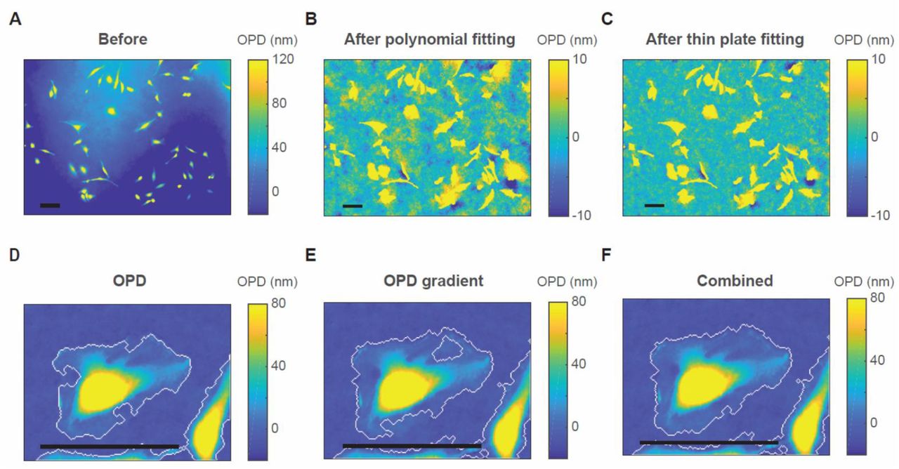
Background subtraction. (A) The OPD image before background subtraction. (B) The OPD image after subtracting the background fitted by a 2D polynomial (n = 8). (C) The OPD image after subtracting the background fitted by the thin plate spline. (D, E) Cell boundaries determined by a threshold on the OPD images (D)or the gradient magnitude of the OPD image (E). (F) The combination of the boundaries on (D) and (E). (A-C) are from a FOV under 10X objective lens. (D-F) are from a FOV under 40X objective lens. Scale bars indicate 100 µm.
We first isolate the objects from the background by “top-hat filtering”. A disk-size smaller than most of the cells is chosen as the structuring element to clean up the fluctuations whose scale are comparable to or larger than the cells. The resultant image cannot be directly used for quantification because it subtracts excessive background from the cells and the mean of the background level is not stable. We only use it to isolate the objects. Then we segment the image to cells and the cell-free area by combining the filtered OPD image and its gradient magnitude to define the boundary of the cells. Thresholding OPD or OPD gradient alone leaves out part of the very thinnest edge of the cell (Fig. 2D and E), but the combination of the two accurately detects the cell boundaries (Fig. 2F). Note that we intentionally do not fill the holes in the masks as other QPM segmentation methods recommended(18, 30), because this process may also fill the blank area within a cell cluster, which is critical for the precise fitting. Lastly, we create the background image by fitting the cell-free area of the original image by the thin plate spline method(31). A mesh grid binning is used for fast calculation. The thin plate fitting is parameter free and can capture both large and small curvatures. Fig. 2C shows that our method generates a cleaner background than conventional methods.
The precision of dry mass measurements
The dry mass measurement error contains all the variation in the OPD measurement, the background subtraction, and the cell segmentation. Among those factors, the background subtraction has the largest effect, as the unevenness in the background affects the cell boundaries. We quantified the precision of the dry mass measurement using fixed cells. The result is summarized in Table 1. Our background subtraction algorithm significantly reduces the dry mass measurement error. The precision is improved at all magnifications when compared to a previous study(18). The algorithm works especially well at low magnifications: the error at 10X is reduced by more than two-fold. Although the OPD noise decreases with magnification, the dry mass measurement error does not change as much. The error at 10X is only 1.16-fold higher than at 20X, while the FOV is four-fold larger. With these improvements of precision at low magnification, we optimized the data collection to maximize throughput at 10X.
Dry mass measurement precision at different magnifications.
Cell segmentation and cell tracking
For cell segmentation, the watershed algorithm works the best when a nuclear marker is used as the foreground marker(32). When no nuclear marker is available, we use the local maximum of the cell after top-hat filtering. Because two cells may closely contact each other and form only one local maximum or one cell may have two local maxima, segmentation without any nuclear marker possesses about 5% error depending on cell types. We combine the OPD image and its gradient magnitude to define the boundary of the cells as discussed in Background leveling corrections.
To track cell trajectories in time automatically, we first identify all the mitotic cells in the time series based on their rounded morphology, by their mass density gradient and area (Fig. 3A). We then trace cells backward. Each track starts from the end of the time series or a mitotic event. No new track is added during the tracing process. We use cell mass, area, and centroid position as the metrics for tracing. We compare a cell k on frame i with each cell on frame i − 1 by the weight function:
 where d is the distance between the centroids, rm is the relative mass difference, ra is the relative area difference, j indicates when the metrics of cell k are lastly updated, and wD, wM, wA, and wG are the weights of the respective terms. The dry mass measurement is so precise that we can put high confidence in the mass term. The weight parameters for HeLa are summarized in Table 2, as an example. The value of W is used to determine the goodness of the match. A good match shall have the smallest W on the frame and W<1. When cell k has a good match, its metrics are updated with the newly traced cell. Otherwise, the old metrics are carried on to be compared with the next frame. This method may leave gaps in tracks that can be filled later by the smoothing algorithm, but tolerate most of the segmentation error. The track doesn’t terminate or deviate by the wrong segmentation of a single frame. A track essentially terminates when it cannot find a good match for more than ten frames (j − i + 1) ∗ wG > 1. In the last step, we trace the lineages of the cells. We compare the metrics at the end of each track with all the mitotic cells. If a track ends just before a mitotic event (the time axis is inverted), the centroid position is near the position of the mitotic cell and the mass is close to half of the mitotic mass, the track is identified as the daughter cell of the mitotic cell. Because newborn cells tend to closely contact their sisters, this will result in an problematic segmentation. For that reason, many cells cannot be traced back to the very beginning of birth. For consistency, we use the division time (the last frame of mitotic rounding) of the mother cell as the birth time of the daughter cells.

Cell tracking. (A) The gradient magnitude of an OPD image measured at 10X. Scale bar indicates 20 µm. The arrow indicates a mitotic cell. (B) One cell is traced to its granddaughter cells. Each color represents a cell. Solid dots are the raw data of dry mass measurement. Solid lines are the spline line smoothing. Vertical dashed lines indicate the timing of cell divisions. Dash-short dash lines indicate the timing of G1/S transitions. (C) The intensity of Geminin-GFP measured in one cell (blue) and its logarithm (red). Dash-short dash line indicates the steepest slope of the log(Geminin-GFP) accumulation curve, which is defined as the timing of G1/S transition.
Fig. 3B shows an example of a cell traced to its grand-daughter cells. For each cell, the G1/S transition is determined by the steepest slope of log(Geminin-GFP) accumulation curve (Fig. 3C). Using the methods described above we were able to successfully trace the cells in a completely automated fashion without manual supervision or correction. We routinely identified and measured more than 10,000 single cell tracks from 432 FOVs of 1.2 mm X 0.9 mm in a 48-hour experiment. The mistraced cells are less than 2%. The limit of the measurement throughput is the speed we can move the stage without perturbing the optical stability of the culture medium surface.
The weight parameters to track HeLa cells.
Detection of growth rate convergences
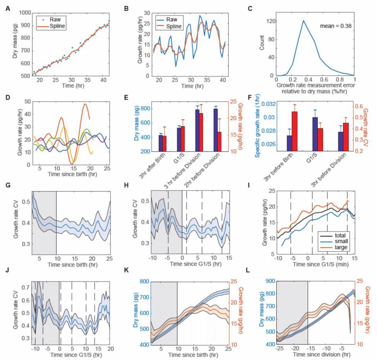
We examined the mass versus time data of about 30,000 cells from three replicate experiments. To each of the single-cell dry mass trajectories, we applied the cubic smoothing spline to fill any gaps and filter the noise (Fig. 4A). We then fitted the growth by a linear model with a 3-hour sliding window along the trajectory. The center time point of the sliding window is recorded as the time when the growth rate was measured. The spline smoothing reduces the random noise in the growth rate trajectory but retains major fluctuations (Fig. 4B). The measurement error of the growth rate is 0.38% mass per hour, as estimated by applying the same measurements and data processing to fixed cells (Fig. 4C). When cells double their mass every 25 hours in an exponential manner, the dry mass increase by 2.77% mass per hour on average. Thus 0.38% mass per hour growth rate accuracy translates to 13.7% accuracy of growth rates. However, this estimate does not include the error caused by erroneous segmentation. When cells are in contact or overlap, it is impossible to draw a true 2D boundary between the cells. Moreover, with our experimental settings, the measurement error in the rounded cells is higher than that in the spread cells, due to the change of focus and the error in phase unwrapping. Thus, to get the most accurate growth rate measurement, we took advantage of the high throughput and discarded any data points where cells were in contact or rounded. In the end, we collected several hundred growth rate trajectories covering the full cell cycle from three independent experiments. The trajectories do not contain the first 1.5 hour after birth and the last 0.5 hour before division due to the removal of attached cells and rounded cells, respectively.

(A) An example of the single-cell dry mass trajectories. (B) The growth rate trajectories of (A) fitted by a linear model with a 3-hour sliding window. (C) The distribution of the growth rate measurement error relative to the dry mass of the cell, estimated from fixed cells. (D) Examples of single-cell growth trajectories synchronized to birth. Each color represents a cell. (E) The average of dry mass and growth rate in the population at specific times of the cell cycle. (F) The average of the specific growth rate and growth rate CV in the population at specific times of the cell cycle. Error bars indicate the standard deviation of three replicative experiments (E, F). (G, H) The growth rate CV changes with time when the trajectories are synchronized to birth (G) or G1/S (H). (I) The mean growth rate of all the cells (black), the top one-third (red) large cells, and the bottom one-third small cells (blue) when the trajectories are synchronized to G1/S. The cells are sorted based on their dry mass at G1/S. (J) The growth rate CV at 33°C when the trajectories are synchronized to G1/S. Dash lines indicate the convergences of growth rate (H-J). (K, L)The mean of dry mass and growth rate when the trajectories are synchronized to birth (K) or division (L). The colored shaded regions indicate the 95% confidence intervals (G, H, J, K, and L). The gray shaded regions indicate the average G1 phase (G, K, and L) or G1 phase (H and J).
Fig. 4D shows examples of several growth rate trajectories. As the individual trajectories are complex, we focused on the mean behavior of the population. We found that growth rate increases with cell mass progressing through the cell cycle except for a rapid decrease just before division (Fig. 4E). We also found that the specific growth rate (growth rate divided by mass) peaks at G1/S, while the growth rate CV is then at its lowest level (Fig. 4F). This is consistent with a previous study done in suspension cells by SMR method(7). The average growth rate CV we measured in HeLa cells is about 40%, which is systematically higher than the about 15% CV observed in suspension cells(7). As our measurement error is much smaller than the average CV, it should not be the dominant factor of the observed variation. The growth rate CV we measured reflects the true cell-to-cell variability.
To understand why the growth rate CV is lowest at G1/S, we further investigated how the growth rate CV changes with time. No effect of environmental fluctuation should induce any synchronized behavior since the averaging was done on an asynchronous population by in silico registration of the individual growth rate trajectories to a particular time in the cell cycle (also known as in silico synchronization). But if the regulation of growth rate were coupled to specific cell cycle stages and the cell trajectories were plotted by in silico synchronization, then we might expect to detect growth kinetics linked to the cell cycle position. We indeed found, as described by Son et al. in suspension cells, that the growth rate CV is highest at birth followed by a rapid drop (Fig. 4G). In addition, the growth rate CV drops several times throughout the cell cycle, particularly at G1/S. There are four recognizable dips when cells are synchronized to G1/S: approximately one in early G1, one at G1/S, one in S phase, and one in G2 phase. The average interval is about 5.8 hours (Fig. 4H). Furthermore, we found that the large cells slow down and the small cells speed up at the dips (Fig. 4I), resulting in growth rate convergences, which could serve as a key mechanism of size control.
We next investigated whether the growth rate convergences are coupled to specific cell cycle stages and whether they take place at a specific frequency. When we grew the cells at 33°C, the average cell cycle elongated from 25.5 hours to 31 hours. Curiously, we found six recognizable dips in total within an average cell cycle under this condition (Fig. 4J). The average interval is 4.7 hours. Thus, the convergences of growth rate seem not to be associated with specific cell cycle stages. The occurrence may therefore be periodic. One possible explanation of the periodic convergence is that the fluctuation in growth rate is periodic, with the phases in large and small cells, shifted. Since the large and small cells spend different times in each cell cycle state, their phase difference may change if we synchronize the trajectories to different cell cycle events. Indeed, the phases of the growth rate fluctuation become better aligned when synchronized to birth or division and this reveals more clearly that the periodicity shows up in the mean growth rate (Fig. 4 K and L). The periodicity is even more apparent in the specific growth rate or the first time derivative of growth rate, as both diminish the effects of the proportionality between growth rate and cell mass (Fig. S1C-F). Since spurious oscillations are found in many closely observed mechanical processes we want to reinforce the fact that the cell trajectories were from cells that were born at different times and subsequently computationally aligned. Thus it is hard to see how this periodicity could have arisen from environmental fluctuation or some collective signal among cells. Indeed, the periodicity is not found in the mean specific growth rate at birth (Fig. S1G) or the growth rate in fixed cells (Fig. S1H). It is found in all the three replicate experiments (Fig. S1I) and it is not induced by the smoothing method (Fig. S1J). Thus we conclude that the periodic fluctuation is intrinsic to the growth rate and may hold a key for understanding size homeostasis.
Discussion
It has been long suggested that QPM should be applicable to a high throughout, longitudinal study of cell mass and growth rate(13). A number of previous studies have demonstrated the possibility of measuring cell growth in several hundred cells for several hours to days(17, 24, 33, 34). However, there is a substantial gap between the demonstration and practical applications. Some of the studies manually segmented and tracked the cells(24, 34), and none of them considered the effect of segmentation error on the growth rate measurement. Here, we developed the QPM system based on a commercial QWLSI camera, which is compatible with a low coherent light source and fluorescence detections. We systematically designed the methods to generate the reference phase image for a variety of sample configurations, especially for multiple-well plates usually used in large-scale screenings. We improved the algorithm for background subtraction and made the measurement precision at low magnification nearly as good as at high magnifications, thus facilitating high throughput data acquisition. Finally, we developed the software for completely automated cell segmentation and cell tracking, making the image processing of large data sets possible. In summary, we made the high throughput, longitudinal measurement of cell mass and growth rate, more precise, practical and convenient. The system can be adopted into broad applications from the fundamental study of cell size and growth rate regulation to large-scale screening for clinical proposes.
It has only been recent that reasonably accurate measurements of growth rate have been possible(7, 14, 17, 24, 25). When observed at high sensitivity, single cell growth rate trajectories are complex. The fluctuations in individual growth rate trajectories embody rich information about the stochastic processes in the cell and potential anabolic and degradative regulation related to progression through the cell cycle. The increased definition of the growth rate plots extracted from single cell trajectories produces new features that are not expected from simple cell cycle models. Fitting these growth trajectories with a simple linear or exponential model averages out the meaningful fluctuations. Furthermore, the simplified models are not good fits, i.e. well below the precision of the measurements. The failure of the simplified models posed the question to us of how to extract the potentially rich information from single cell trajectories. Many previous studies investigated the correlations between growth rate and cell mass(7, 24, 25), which makes sense in terms of the long debate between the linear and exponential growth models. However, this type of analysis ignores “cell cycle time” in the regulation. For the investigation of the cell-cycle controlled regulation, given the inherent variation in cell cycle length, the question emerges as how to synchronize the cells (whether experimentally or by in silico analysis from single-cell data). A few studies, emphasizing the importance of the G1/S transition in cell cycle commitment, synchronized the trajectories to G1/S, assuming that the cell-cycle dependent growth rate regulation is also regulated at the G1/S transition(7). But different forms of synchrony will, in general, produce different behaviors. We recommend synchronizing the trajectories to several cell cycle events, since feedback could occur in any stage of the cell cycle. Furthermore, the numerical analysis of the growth can reveal different features, so it is worthwhile to use various functional forms, from the linear growth rate (the mass change per unit of time), the specific growth rate (growth rate divided by mass), as well as the first derivative of growth rate (the acceleration or deceleration of growth rate), since different forms have power to reveal different regulative mechanisms.
In 2013, Kafri et al. first discovered size-dependent growth rate modulation in adherent mammalian cells(4). They measured the cell mass of millions of fixed cells from an asychronized population and interpreted dynamics from the measurements by using and analytical approach, which they called Ergodic Rate Analysis. They found that the correlation between cell size and growth rate becomes negative in late G1 and S phase. The mean growth rate of the population also slows down at the two corresponding times. The study cannot rule out that the growth rate regulation in early G1 or G2 phase is due to the cell cycle markers, which lacked sufficient time resolution in those phases. In their analysis a decrease in growth rate could be due to a slowdown in protein accumulation or equally an acceleration of passage through the cell cycle. Later, Ginzberg et al. discovered three dips in HeLa cells in the apparent growth rate CV, Gcv, by combining live cell and fixed cell measurements(5). The dips were at approximately 4, 10 and 16 hours after birth, i.e. at 6-hour intervals. Both studies seemed to extract accurate information from the mean behavior of a large population, and suggest that the growth rate modulation plays an important role in maintaining size homeostasis. However, artificial synchronization could produce artifacts and up to now there has been no evidence obtained from direct measurements of individual cell growth rate over long time periods. The QPM methods and forms of analysis reported here measured single cell growth rates in adherent mammalian cells to the accuracy of 13.7%. We convincingly found four dips in the growth rate CV throughout the cell cycle caused by or possibly causing the growth rate convergence in large and small cells. The timing and interval of the dips are surprisingly consistent with the ones discovered by Kafri et al. and Ginzberg et al. by completely different methods. Furthermore, we found the dips are not coupled to specific cell cycle stages, and instead may take place at a certain frequency.
Before speculating further, we wish to emphasize that we are well aware that periodic variation could be spurious. In any experimental setting, these could be induced by fluctuations in the environment particularly if they coincided with natural variation, as temperature, light, line voltage, O2, CO2, etc. But we point out that although later synchronized in silico, these cells were asynchronously growing so that the experimental time bears no relationship to real time and the individual members of the population can be expected to be scrambled with respect to time in each experiment. We therefore believe that the periodicity is intrinsic to growth rate regulation. And, the CV reduction may be caused by the phase shift between the large and small cells. Usually, an oscillation is caused by negative feedback with a substantial time delay(35). These oscillations most sensitively seen in growth rate acceleration suggest novel underlying mechanism of growth rate modulation and may pave the road to the mechanistic studies. It suggests an interest in searching for corresponding oscillatory circuits in protein synthesis/degradation, activity or inactivity of signaling pathways either tied to or independent of anabolism and catabolism, and perhaps tied to other cellular funcitions. Such mechanisms may function to maintain homeostasis by differentially affecting cells of different size. It would be interesting to look at the size variability of cells arrested in the cell cycle. Since the growth rate corrections are not associated with specific cell cycle stages and rather occur at a given frequency, we might expect size variability to be restrained by repeated episodes of growth rate correction, even as the arrested cells continue to grow.
Materials and Methods
Cell culture
HeLa Geminin-GFP cells were generated and single clones were isolated and grown in our laboratory. Cells grown in Dulbecco’s Modification of Eagles Medium (DMEM, ThermoFisher Scientific, 11965), supplemented with 10% Fetal Bovine Serum (FBS, ThermoFisher Scientific, 16000044), 5% penicillin/streptomycin (10000 U/mL, ThermoFisher Scientific, 15140122), 10 mM sodium pyruvate(100 mM, ThermoFisher Scientific, 11360070), and 25mM HEPES (1 M, ThermoFisher Scientific, 15630080), were incubated at 37°C with 5% CO2.
Microscope setup
The SID4BIO camera (Phasics, France) was integrated into a Nikon Eclipse Ti microscope through a C-mount. For QPM imaging, we used a halogen lamp as the transmitted light source. A Nikon LWD N.A. 0.52 condenser was used with the aperture diaphragm closed. A C-HGFI mercury lamp was used for fluorescence illumination. A Nikon TI-S-ER motorized stage was used to position the sample with the moving speed of 2.5 mm/s in XY direction (accuracy 0.1 µm). A Nikon Perfect Focus System (PFS) was used for maintaining the focus. An Endow GFP/EGFP filter sets (Chroma 41017) was used to take the Geminin-GFP image. We used three objective lenses as indicated in this study, one Nikon Plan Flour 10X N.A. 0.3 PFS dry, one Nikon Plan Apo 20X N.A. 0.75 PFS dry, and one Nikon Plan Apo 40X N.A. 0.95 PFS dry. NIS-Elements AR ver. 4.13.0.1 software with the WellPlate plugin was used to acquire images. A homemade incubation chamber was used to maintain the constant environment of 36°C or 33°C and 5% CO2.
Quantification of measurement errors
To quantify the OPD noise of the blank sample, we performed all the measurements as described on the blank 6-well glass-bottom plates filled by Phosphate-Buffered Saline (PBS, Corning, 21-040-CV) and mineral oil (Sigma-Aldrich, M8410) at 10X magnification.
Fixed cells were used to quantify the dry mass and growth rate measurement error. For sample preparation, cells were seeded in 6-well glass-bottom plates (Cellvis, P06-1.5H-N) at 3500 cells/cm2 overnight, then fixed in 0.2% glutaraldehyde (50 wt. % in water, Sigma-Aldrich, 340855) for 10 min at room temperature. Then the fixed cells were immersed in PBS and topped with mineral oil.
In the experiments to quantify the dry mass measurement error, cells were imaged every 5 min for 2 hours. At 10X magnification, an area of 8×8 FOVs in the well center was scanned, with the X-Y step distance as one-fifth of the FOV. At 20X, an area of 15×15 FOVs was scanned, with one-fifth of the FOV as the step distance. At 40X, 60 cells were chosen manually; each was imaged in four FOVs with the cell at a different corner. The temporal error was quantified as the standard deviation of the time series of each cell divided by the mean mass of the cell. To quantify the net spatial error, we averaged the dry mass measurements through the time series first to eliminate the error caused by the temporal variation, then took the standard deviation divided by the mean of each cell at different positions as the spatial error. The temporal and spatial combined error was the standard deviation divided by the mean of each cell at different positions without averaging by time series.
In the experiments to quantify the growth rate measurement error, the fixed cells were imaged and analyzed as in the long-term live cell experiments. The standard deviation of the growth rate of each cell was taken as the growth rate measurement error and normalized by the mean mass of each cell. The mean of the resultant distribution was taken and divided by the percentage of the mass increase per hour. The result is the relative measurement error of the growth rate.
Long-term live cell imaging
The 6-well glass-bottom plates were treated by Plasma Etcher 500-II (Technics West Inc.) at 75 mTorr, 110 W, for 1 min, then coated by 50 µg/mL fibronectin (Sigma-Aldrich, F1141) overnight. Cells were seeded on the pre-coated plates at 2000 cells/cm2 3 hours prior to the experiments in the medium of DMEM without phenol red (ThermoFisher Scientific, 21063) supplemented with 10% FBS, 5% penicillin/streptomycin, and 10 mM sodium pyruvate, and topped with mineral oil. All the experiments were done at 10X magnification. The Phase images were acquired every 30 min, and the fluorescent images were acquired every 1 hour, at 36°C for 48 hours or at 33°C for 72 hours by the SID4BIO camera. The position of the FOVs was generated by a custom developed GUI in Matlab (MathWorks), which assured that the FOVs were within the center 10% area of the well and were evenly spaced. 72 FOVs were imaged in each well.
Image analysis and data analysis
When needed the performance of the reference and parameters for segmentation were evaluated by a custom-developed GUI. All the image processing pipeline (generating the reference wavefront, applying the reference, background subtraction, cell segmentation, and cell tracking) was conducted on a high performance compute cluster by custom-written codes in Matlab. The last 2 hours of the growth rate trajectories were truncated when they are synchronized to birth or G1/S to avoid the effect of the sudden growth rate slowdown before division. The 95% confidence intervals of the mean were calculated as  where n is the data number, SEM is the Standard Error of the Mean
  . The 95% confidence intervals of CV were calculated as
  .
.
Acknowledgment
We thank the Nikon Imaging Center at Harvard Medical School for their courtesy in sharing space and other resources. We thank the National Institute of General Medical Sciences for support (5RO1GM26875-42). All the image processing, data transfer, and data storage were conducted on the O2 Compute Cluster, supported by the Research Computing Group at Harvard Medical School. The plasma treatment was done at the HMS Microfluidics Core Facility.
References


