

Abstract
Microbial communities can evade competitive exclusion by diversifying into distinct ecological niches. This spontaneous diversification often occurs amid a backdrop of directional selection on other microbial traits, where competitive exclusion would normally apply. Yet despite their empirical relevance, little is known about how diversification and directional selection combine to determine the ecological and evolutionary dynamics within a community. To address this gap, we introduce a simple, empirically motivated model of eco-evolutionary feedback based on the competition for substitutable resources. Individuals acquire heritable mutations that alter resource uptake rates, either by shifting metabolic effort between resources or by increasing overall fitness. While these constitutively beneficial mutations are trivially favored to invade, we show that the accumulated fitness differences can dramatically influence the ecological structure and evolutionary dynamics that emerge within the community. Competition between ecological diversification and ongoing fitness evolution leads to a state of diversification-selection balance, in which the number of extant ecotypes can be pinned below the maximum capacity of the ecosystem, while the ecotype frequencies and genealogies are constantly in flux. Interestingly, we find that fitness differences generate emergent selection pressures to shift metabolic effort toward resources with lower effective competition, even in saturated ecosystems. We argue that similar dynamical features should emerge in a wide range of models with a mixture of directional and diversifying selection.
Ecological diversification and competitive exclusion are opposing evolutionary forces. Conventional wisdom suggests that most new mutations are subject to competitive exclusion, while ecological diversification occurs only under highly specialized conditions (1). Recent empirical evidence from microbial, plant, and animal populations has started to challenge this assumption, suggesting that the breakdown of competitive exclusion is a more common and malleable process than is often assumed (2, 3, 4). Particularly striking examples have been observed in laboratory evolution experiments, in which primitive forms of ecology evolve from a single ancestor over years (5), months (6), and even days (7).
In the simplest cases, the population splits into a pair of lineages, or ecotypes, that stably coexist with each other due to frequency-dependent selection, leading to a breakdown of competitive exclusion (5, 6, 8, 9, 10). But evolution does not cease after ecological diversification occurs. Instead, recent sequencing studies have shown that adaptive mutations continue to accumulate within each ecotype, even when population-wide fixations are rare (11, 12, 13). This additional evolution can cause the ecological equilibrium to wander over longer timescales, as observed in the shifting population frequencies of the two ecotypes (5, 13). In certain cases, these evolutionary perturbations can even drive one of the original lineages to extinction, either through the outright elimination of the niche (9), or by the invasion of individuals that mutate from the opposing ecotype (12).
Pairwise coexistence is the simplest form of community structure, but similar dynamics have been observed in more complex communities as well. Some laboratory experiments diversify into three or more ecotypes (7, 14, 15), and it is likely that previously undetected ecotypes may be present in existing experiments (13). Moreover, many natural microbial populations evolve in communities with tens or hundreds of ecotypes engaged in various degrees of competition and coexistence (16, 17, 18). Although the evolutionary dynamics within these communities are less well-characterized, recent work suggests that similar short-term evolutionary processes can occur in these natural populations as well (19, 20, 21).
While the interactions between microbial adaptation and ecology are known to be important empirically, our theoretical understanding of this process remains limited in comparison. Early work in the field of adaptive dynamics (22) showed how ecological diversification emerges under very general models of frequency-dependent trait evolution, which are thought to describe the limiting behavior of a wide class of ecological interactions near the point of diversification. Numerous studies have also investigated the effects of evolution on ecological diversification and stability using computer simulations, in which the parameters of a particular ecological model are allowed to evolve over time (23, 24, 25, 26, 27, 28, 29). However, while both approaches can reproduce some of the qualitative behaviors observed in experiments, it has been difficult to forge a more quantitative connection between these models and the large amount of molecular data that is now available.
One of the main reasons why quantitative comparisons have been difficult is that in many microbial populations of interest, natural selection acts on a range of traits in addition to those directly involved in diversification. The mutations that influence ecological phenotypes must therefore compete with constitutively beneficial mutations at unrelated loci, which can often comprise the bulk of the observed mutation events (12, 13). Although many models exist for describing these constitutively beneficial (or deleterious) mutations in the absence of ecology (30), we have few quantitative predictions for how they behave when they are linked to ecological phenotypes, and vice versa. This makes it difficult to draw any quantitative inferences from the vast molecular data that is now available.
To start to bridge this gap, we introduce a simple, empirically motivated model that describes the interplay between ecological diversification and directional selection at a large number of linked loci. The ecological interactions derive from a well-studied class of consumer resource models (31, 32, 33, 34), in which individuals compete for multiple substitutable resources (e.g. different carbon sources) in a well-mixed environment. We extend this ecological model to allow for heritable mutations in resource uptake rates, which can either divert metabolic effort between resources, or the increase overall fitness. The latter class of mutations provides a natural way to model adaptation at linked genomic loci.
These constitutively beneficial mutations might seem like an ecologically trivial addition to the model, since they are always favored to invade on short timescales. On longer timescales, however, we will show that these accumulated fitness differences can dramatically influence both the ecological structure and the evolutionary dynamics that take place within the community. By focusing on the weak mutation limit, we derive analytical expressions for these dynamics in the two resource case, and we show how our results extend to larger communities as well. These analytical results provide a general framework for integrating ecological and population-genetic processes in evolving microbial communities, and suggest new ways in which these processes might be inferred from time-resolved molecular data.
EVOLUTIONARY MODEL OF RESOURCE COMPETITION
To investigate the interactions between ecological diversification and directional selection, we focus on a simple ecological model in which individuals compete for an assortment of externally supplied resources in a well-mixed, chemostat-like environment (Fig. 1). This resource-based model aims to capture some of the key ecological features observed in certain microbial evolution experiments (5, 8), as well as more complex ecosystems such as the gut microbiome (18), while remaining as analytically tractable as possible.

(a) Schematic depiction of ecological dynamics. Substitutable resources are supplied to the chemostat at constant rates  , measured in units of biomass
  . Cells import resources at genetically encoded rates, ri, which define a normalized resource strategy
  and general fitness
  . (b) Schematic depiction of evolutionary dynamics. Mutations that alter resource strategies
  occur at rate Uα, while mutations that alter general fitness (X) occur at rate UX. (c-f) Simulated ecological and evolutionary dynamics, starting from a clonal ancestor, in an environment with
  resources. The four panels represent independent populations evolved under different sets of parameters, which differ only in the mutation rates and fitness benefits of pure fitness mutations (SI Appendix E). Lines denote the population frequency trajectories of all mutations that reached fequency ≥ 10% in at least one timepoint. Resource strategy mutations are shown in red, while pure fitness mutations are shown in blue.
In our idealized setting, individuals compete for  substitutable resources, which are supplied by the environment at a fixed rates (Fig. 1). Individuals are characterized by a resource utilization vector
  , which describes how well they can grow on each of the resources. We assume that the resource utilization phenotypes are constitutively expressed, so that we may neglect complicating factors like regulation. We will find it useful to decompose the phenotype
  into a normalized portion
  , and an overall magnitude
  , where
  is an arbitrary dimensionful constant. The components of
  can be interpreted as the fractional effort devoted to growth on resource i, and we will refer to this quantity as the resource strategy vector. In contrast, the magnitude X resembles an environment-independent measure of general fitness, an analogy that we will make more precise below.
We assume that individuals reproduce asexually, so that the state of the ecosystem can be described by the number of individuals nμ with a given resource strategy vector  and fitness Xμ. Under suitable assumptions, the ecosystem can be described by the coarse-grained Langevin dynamics,
 where N is a fixed carrying capacity, fμ = nμ/N is the relative frequency of strain μ, and ξμ(t) is a stochastic noise term (SI Appendix A). The state of the environment is encoded by the set of resource-specific mean fitnesses,
 where βi denotes the fractional flux supplied by resource i. Eq. (1) is an example of a more general and well-studied class of consumer resource models introduced by Refs. (31, 35), whose ecological properties have been explored in several recent works (32, 33, 34). The same equation also describes a “bet-hedging” scenario in which the population is periodically subdivided into different environments (SI Appendix A). For a single resource, Eq. (1) reduces to the standard Wright-Fisher model of population genetics (36), with its logistic growth function, ∂t log
  . The parameter Xμ can therefore be identified with the (log) fitness in these models. In a multi-resource environment, the deterministic dynamics become more complex, and do not generally admit a closed form solution for fμ(t). However, Eq. (1) still possesses a convex Lyapunov function (SI Appendix A), which implies that fμ(t) must reach a unique and stable equilibrium at long times.
The ecological model in Eq. (1) describes the competition between a fixed set of strains. To incorporate evolution, we also allow for new strains to be created through the process of mutation. We will show that it is useful to distinguish between two broad classes of mutations. The first class, which we will refer to as strategy mutations, alter the resource uptake strategy  , while for simplicity, leave the general fitness X unchanged. We assume that these mutations occur at a per genome rate Uα and result in a new resource strategy
  drawn from some distribution
  . In addition to these strategy mutations, we consider a second class of pure fitness mutations, which alter the general fitness X but leave the resource strategy
  unchanged. These mutations capture the effects of directional selection at a large number of other loci throughout the genome, which may only be tangentially related to the resource utilization strategy. We assume that these fitness mutations arise at a per-genome rate UX, and that they increment X by an amount s drawn from the distribution of fitness effects, ρX(s). For simplicity, we assume that there is no macrosopic epistasis for fitness (37), so that ρX(s) remains the same for all genetic backgrounds.
This division into fitness and strategy mutations is neither exhaustive nor unambiguous. Some changes in resource strategy may also incur a fitness cost, and one can simulate a pure fitness mutation by shifting metabolic effort away from resources that are not present in the current environment (i.e., those with βi =0). Nevertheless, by considering these as independent axes, we will show that we can gain additional insight into the behavior of our model.
Pure fitness mutations might seem like an ecologically trivial addition to the model, because they are always favored to invade. However, computer simulations show that these accumulated fitness differences can still have a dramatic influence on both the ecological structure and the evolutionary dynamics that arise in a given population. Figures 1C-F depict individual-based simulations of four populations, which are subject to the same environmental conditions and the same supply of strategy mutations, but have different values of UX and ρX(s) (SI Appendix E). Depending on the supply of fitness mutations, the behaviors range from rapid diversification and stasis (Fig. 1C) to unstable but continually renewed coexistence (Fig. 1D), stable coexistence and rapid within-clade evolution (Fig. 1E), and the permanent disruption of coexistence (Fig. 1F).
To understand these different behaviors and their dependence on the underlying parameters, we will start by analyzing the simplest non-trivial scenario, in which the strains evolve in an environment with just two resources. In this case, the environmental supply rates and resource uptake strategies can be described by scalar parameters  and
and  , respectively. This case will already be sufficient to elucidate many of the key qualitative behaviors and fundamental timescales involved, while maximizing analytical tractability. In the second section, we will extend this analysis to larger numbers of resources, and comment on the additional features that arise only in this more complicated scenario.
ANALYSIS
Selection for ecosystem to match environment, stable coexistence
We will begin by considering the dynamics in the absence of fitness differences (UX = 0, Xμ = 0). The ecological dynamics in this “neutral” scenario have recently been described by Ref. (32), and it will be useful to build on these results in the sections that follow.
We begin by considering a single strategy mutation that occurs in a clonal population of type α1, creating a new strain of type α2. The initial dynamics of this mutation can be described by a branching process with growth rate Sinv = 〈∂tf〉/f (SI Appendix B), also known as the invasion fitness. In this case, the invasion fitness is given by
 where Δα = α2 – α1 is the difference between the mutant and wildtype uptake rates. The invasion fitness is positive whenever Δα and β – α1 have the same sign: if α1 > β, then selection will favor mutations that increase α, while if α1 > β, selection will favor mutations that decrease a. In this way, selection tries to tune the population uptake rate to match the environmental supply rate. If α1 = β, then the invasion fitness vanishes for all further strategy mutants. This constitutes a marginal evolutionarily stable state (ESS). It will turn out that many expressions simplify in a near-ESS limit, where the uptake rates ai remain close to β. We will focus on this regime for the expressions quoted in the remainder of the main text, while the full expressions are derived in SI Appendix.
Since all mutations start as a single copy in the population, many will be lost due to genetic drift, even when they are favored by selection. With probability ~Sinv, the mutant lineage will survive to reach frequency f ~ 1/NSinv, and will then start to increase determin-istically; in large populations, this will typically occur long before the mutant starts to influence its own growth rate, so that the constant invasion fitness assumption is justified (SI Appendix B).
At long times, the ecological dynamics will lead to one of two final states: the mutant will either replace the wildtype (competitive exclusion) or the two will coexist at some intermediate frequency (Fig. 2A). The latter scenario will occur if and only if the wildtype can re-invade a population of mutants, which requires that the reciprocal invasion fitness,  , is also positive. By examining this expression, we see that the mutant will outcompete the wildtype if its strategy lies between β and α1, while stable coexistence occurs when α1 and α2 span β (i.e., α1 < β < α2 or vice versa). When this condition for coexistence is met, Ref. (32) has shown that the steady-state frequencies are determined by the linear equation,
 whose solution is given by f*/(1–f*) = (β–α2)/(α1 – β). In other words, the relative frequencies of the strains are inversely proportional to their distance from the environmental supply rate. According to Eq. (4), these frequencies are chosen such that the population-averaged uptake rate
  exactly balances the resource supply rate β. This provides an intuitive explanation for the cause of coexistence: by maintaining the strains at intermediate frequencies, the population is able to match the environmental supply rate more closely than it could with either strain on its own.

(a) Ecological diversification from a clonal ancestor. In the absence of fitness mutations, strains coexist at a stable equilibrium (f*) with fluctuations (δf) controlled by genetic drift. Further strategy mutations are not favored to invade. (b) Pure fitness mutations that sweep within an ecotype shift the stable equilibrium by Δf; accumulated fitness differences can ultimately drive ecotypes to extinction. Further strategy mutations allow the winning clade to re-diversify at a later time. (c) Occupied niches can also be invaded by strategy mutations that arise in fitter genetic backgrounds. In this case, the original ecotype lineage is driven to extinction while the ecological structure of the community is preserved.
Once this ecological equilibrium is attained, number fluctuations will continuously perturb the true frequency away from f* (Fig. 2A), subject to a linearized restoring fitness ~Δα2/β(1 – β) (SI Appendix B). The restoring force is strong compared to genetic drift when NΔα2/β(1 – β) ≫ 1, which leads to linearized fluctuations of order  , and a lifetime for the stable state that is exponentially long in
  . At this point, additional strategy mutants are subject to very weak selection pressures: fluctuations will induce momentary invasion fitnesses of order
  (which can be large compared to 1/N), but these fitness effects are quickly averaged to zero during the ~1/δSinv generations required for such a mutation to establish (SI Appendix B). Thus, once the population diversifies to fill the two niches, the rate of evolution dramatically slows down (as, e.g. in Fig. 1A), since the relevant timescales are controlled by genetic drift. In this way, a large effect mutation can allow the ecosystem as a whole to reach an effective ESS, long before any of the constituent strains reach the ESS on their own.
Diversification load
We are now in a position to analyze how fitness alters the basic picture above. We begin by revisiting the invasion of a mutant strain in an initially clonal population, this time allowing for a fitness difference ΔX between the mutant and wildtype. In this case, the new invasion fitness is given by a simple linear combination,
 where Sinv(Δα) is the invasion fitness for a pure strategy mutation from Eq. (3). This result describes, in quantitative terms, how selection balances its ecological preferences
  with its desire to maximize fitness
  . When the uptake rate of the resident population is far from the environment supply rate
  , the ecological selection pressures can be quite strong, with invasion fitnesses as high as 10% – 100%. This implies that strongly deleterious mutations of order
 can hitchhike to fixation when the population colonizes a new ecological niche (a form of diversification load).
Fitness differences perturb ecological equilibria
In addition to shifting the invasion fitness of a new mutation, fitness differences can also alter the long-term ecological equilibrium between mutant and wildtype in Eq. (4). In the extreme limit, this can disrupt the stable coexistence altogether. If the mutant is less fit than the wildtype (ΔX < 0), this will occur whenever ΔX is less than the maximum diversification load ΔXmin in Eq. (6). On the other hand, if ΔX > 0, extinction will occur when the wildtype no longer has positive invasion fitness, or when ΔX exceeds a threshold

We note that the fitness differences in Eqs. (6) and (7) are lower than the values required for the mutant or wild-type to dominate in all environmental conditions (SI Appendix B). Instead, the fitness thresholds strongly depend on how the resource strategies differ from each other, and from the environmental supply rate. When Δα ~ ϵ, even a small fitness difference (ΔX ~ ϵ2) can disrupt the stable ecology, while for  , much larger fitness differences (ΔX ≳ 100%) can be tolerated.
When ΔXmin > ΔX < ΔXmax, the two strains continue to coexist, but their equilibrium frequency is no longer given by Eq. (4). In this case, the competing drive to maximize fitness means that selection will no longer favor an ecology that matches the environmental resource distribution, at least not perfectly. In SI Appendix B, we show that the new equilibrium frequency is given by
 where
where  is the neutral ecological equilibrium from Eq. (4). From this expression, we can read off the typical fitness differences required to perturb f* from its present value. This fitness sensitivity is again determined by the distance between the two resource strategies. If
  , large fitness differences (ΔX ≳ 100%) are required to change the equilibrium frequency, while for Δα ~ ϵ, even very small fitness differences (ΔX ~ ϵ2) can generate large changes in the equilibrium frequency.
Further fitness evolution and diversification-selection balance
Once the population achieves the stable ecology in Eq. (8), additional fitness mutations will occur in each strain with probability proportional to the equilibrium frequency f*. In our model, the invasion fitness of such a mutation is simply its fitness effect s, independent of the ecological state of the population. With probability ~s, this mutation will sweep through its parent clade, changing the fitness difference between the clades by ±s and the equilibrium frequency by Δf = f*(ΔX±s) –f*(ΔX) (Fig. 2B). In the linear regime of Eq. (8), the frequency and fitness changes are directly related,
 where sc = Δα2/β(1 – β) is the fitness scale that determines changes in equilibrium frequency. If s ≫ scf*(1 – f*), then the stable coexistence will be di srupted, and the mutant clade will take over the population. We will refer to such a scenario as ecosystem collapse, since one of the niches is no longer occupied.
Similar behavior can occur when s ≪ sc as well, except that now the ecosystem collapse occurs due to cumulative effect of many general fitness mutations. When the fitness mutations accumulate independently, this process can be described by an effective diffusion model,
 with a bias that reflects the higher probability of producing a mutation in a larger clade (SI Appendix B). Eq. (10) superficially resembles the drift-induced perturbations at ecological equilibrium, except that the bias is now unstable rather than restoring. When
  , the mutation bias is weak, and the clade frequencies undergo a random walk
  . But after a time of order
  , the frequency differential grows large enough that the more prevalent clade will deterministically produce more beneficial mutations, so that it is destined for fixation. After a time of order
  , the fitness difference between the clades grows so large that the ecosystem finally collapses (Fig. 2B). This timescale sets an upper limit on the lifetime of the stable state when many fitness mutations are available.
Once the ecosystem collapses, there will be a strong selection pressure for the winning clade to re-diversify through additional strategy mutations, and restart this process from the beginning (Fig. 2B). To gain insight into these dynamics, we first consider the case where the resource strategies are controlled by a single genetic locus, with fixed phenotypes α1 and α2, and mutations that alternate between the two states at rate Uα. After an ecosystem collapse, Eq. (3) shows that the invasion fitness for the opposite strategy is given by Sinv ~ sc, so the collapsed state will persist for a time of order τdiversify ~ 1/NUαsc, until the stable ecology is reestablished. If the two strategies are symmetric about β, so that f*(0) = 1/2, the new stable state will persist for ~τcollapse generations in the absence of additional strategy mutations, and the process will then repeat itself. The relative probability of observing the population in the collapsed  or saturated
  states is therefore given by

This expression shows the minimum amount of strategy mutations, or the maximum amount of general fitness mutations, that allow the population to maintain a saturated ecosystem. We will refer to this dynamic steady state as diversification-selection balance, in analogy to mutation-selection balance in population genetics (38). Note that this balance crucially depends on the state of the ecosystem through sc ~ Δα2/β(1 – β). All else being equal, ecosystems with more similar resource uptake strategies will be disrupted more easily than those with a higher degree of specialization.
Invading ecotypes can delay ecosystem collapse
Strictly speaking, our derivation of Eq. (11) is only valid in the limit that τcollapse ≪ τdiversify, since we neglected mutations between α1 and α2 when both niches were filled. When τcollapse ≳ τdiversify (i.e., when the ecosystem spends an appreciable amount of time in the saturated state), we must also account for mutations between the two strategies that arise before the ecosystem collapses. Those mutations that arise in the less-fit clade will have little chance of invading. However, a mutation from the more-fit to the less-fit strategy will establish with probability ~|ΔX|, where ΔX is the current fitness difference between the two clades. If this mutation is successful, it will outcompete the resident lineage with the corresponding value of a, and reset the fitness difference to ΔX = 0 (Fig. 2C). In this way, invasion from one ecotype to another can significantly delay the process of ecosystem collapse, since it relieves the tension between fitness maximization and  and selection to match the environment
  .
.
To analyze this process, we note that successful invasion events will occur as an inhomogeneous poisson process with rate  , where f*(t) and ΔX(t) are again determined by the diffusion model in Eq. (10). This leads to a characteristic invasion timescale
 which is derived in SI Appendix B. Each of these regimes corresponds to a different intuitive picture of the dynamics. In the first case, strategy mutations are frequent compared to general fitness mutations, and invasion occurs almost immediately after the first fitness mutation arises. In the second case, invasion occurs after multiple fitness mutations have accumulated, but when the frequencies of the clades still wander diffusively relative to each other
  . In the third regime, invasion occurs after one of the clades has grown to a sufficiently large frequency that it would have determin-istically led to ecosystem collapse. When the invading mutant establishes, it will therefore cause a rapid shift in the frequencies of the ecotypes as f*(ΔX) returns to f*(0). 2
Finally, when  , strategy mutants are sufficiently rare that the ecosystem will typically collapse and re-diversify before invasion can occur. This sets the region of validity of the diversification-selection balance in Eq. (11). Interestingly, Eq. (11) shows that collapse and re-diversification can still dominate over invasion even when both niches are typically filled
  . In this case, both the genealogical structure and the typical state of the ecosystem will resemble the invasion regime, but the historical record would contain a series of puncutated extinction and diversification events, interspersed with long periods of gradual fitness evolution.
Fitness differences create opportunities for ecological tinkering
Our derivation of Eqs. (10) and (12) assumed that the two ecotypes were fixed by the genetic architecture of the organism. Individuals could mutate between α1 and α2, but mutations to other points in strategy space were forbidden. In the absence of fitness differences, we saw that selection for these additional strategy mutants is weak once both niches have been filled (Sinv ≲ 1/N), potentially justifying the single-locus assumption in terms of a priority effect. However, the previous analysis shows that there can be strong selection to switch strategies once fitness mutations accumulate, so it is also plausible that fitness differences could lead to selection for strategy mutations more generally.
To investigate these selection pressures, we consider a population that is currently described by the steady state in Eq. (8). We then consider strategy mutations that occur on the background of α2, altering its strategy to α3 while leaving its fitness intact. The invasion fitness for such a mutation is given by

As anticipated, fitness differences create additional selection pressure for strategy mutations beyond the simple switching behavior considered above.
The direction of selection is determined by the sign of ΔX. In the background of the fitter clade (ΔX > 0), selection favors mutations that increase the strategy in the direction of β (a form of generalism), while simultaneously disfavoring mutations that lead to increased specialization (Fig. 3). The opposite behavior occurs in the less-fit background, with selection favoring mutations that increase the distance from β, leading to increased specialization. Both behaviors have an intuitive explanation in terms of individuals preferring to allocate their metabolic energy toward the resource with the least-fit consumers, thereby minimizing the effective competition that they experience.

The two resident ecotypes are illustrated by blue circles, while red circles denote mutant strains created by strategy mutations on one of the ecotype backgrounds. The solid black line denotes the effective mean fitness,  , experienced by a given resource strategy. Strains with general fitness (X) above this line are favored to invade, while others are selected against. If a mutant successfully invades, its effect on the ecosystem is indicated by the text.
Once a successful strategy mutation arises, it will sweep through the population and alter the ecological equilibrium (Fig. 3). Mutations in the less-fit clade are straightforward to analyze. Since these are always directed away from both β and α1, these mutants will sweep through their parent clade and increase the equilibrium frequency according to Eq. (8). Successful mutations in the fitter clade have a wider range of outcomes, since these are always directed toward β and α1. If α3 < β, the mutant lineage will outcompete the less-fit strain α1, and will stably coexist with its parent clade α2 at an equilibrium frequency f* = (β – α2)/(α3 – α2). On the other hand, if β < α3 < α2, the mutant lineage will always sweep through its parent clade α2. If α3 is sufficiently close to α2, this will simply lead to an increase in frequency according to Eq. (8). However, if α3 is close enough to β that ΔXmax(α3) becomes less than the actual fitness difference, ΔX, then the mutant will sweep out both clades and lead to an ecosystem collapse and subsequent re-diversification. Thus, in addition to creating a larger target for invasion events, these additional strategy mutations can also enhance the probability of ecosystem collapse. The balance between these competing tendencies will depend on the genetic architecture of the resource strategies, ρα(α’|α), which is poorly parameterized by existing data. A detailed analysis of the potential regimes will be left for future work.
Beyond pairwise coexistence
Our previous analysis focused on environments with only two substitutable resources, where at most two strains can coexist at equilibrium. In this case, the structure of the stable ecosystem was simple enough to admit a full analytical solution, which we could use to derive explicit predictions for many evolutionary quantities of interest. However, many microbial communities are found in environments with large numbers of potential resources, and flexible gene pools that allow them to alter their resource uptake rates through horizontal gene transfer (39). It is therefore natural to ask how our results generalize to these more complicated environments as well. A full analysis of this case is beyond the scope of the present work, as there are even fewer constraints on the space of ecological and evolutionary parameters compared to the two resource case. Nevertheless, it is still useful to know whether our qualitative results extend beyond  , and whether there are fundamentally new behaviors that only arise in higher dimensions.
For a general ecological equilibrium, a mutation that alters the phenotype of a resident strain from  to
to  will have an invasion fitness
 where the resource-specific mean fitnesses
  are given by Eq. (2) evaluated at the equilibrium frequencies
  (SI Appendix C.1). Increases in αi are favored when
  is lower than the “effort-averaged”
  for the other resources, and vice-versa. Thus, similar to the two-resource case, there is still a sense in which selection favors mutations that flow from high values of
  to lower values of
  , though there are now
  beneficial directions,
  , rather than just one.
The invasion fitness in Eq. (14) depends on the current community composition only through the intensive variables  . In a saturated ecosystem, where the number of coexisting strains is equal to the number of resources, these can be directly obtained by a matrix inversion of Eq. (1),
 where
where  is the left inverse of αμ,i. Thus, we see that in a saturated ecosystem, the
  are given by linear combinations of the strain fitnesses Xμ, justifying their interpretation as resource-specific mean fitnesses. Moreover, perturbation expansions of
  suggest that the prefactor is still inversely proportional to an effective distance between the strategies (SI Appendix C.2), similar to the two-resource case in Eq. (13). We note that the equilibrium values of
  are conditionally independent of both the resource supply vector βi and the strain frequencies
  ; these quantities influence
  only through shaping the set of resource strategies that coexist at equilibrium. Thus, these saturated ecosystems dynamically adjust their composition to screen the internal selection pressures
  from the external environmental conditions. Similar findings were recently obtained for the neutral case [where
  (32)], as well as in certain community assembly processes in the
  limit (33, 34). Eq. (15) shows that this is a generic property that occurs whenever the number of surviving species is equal to the number of resources.
In this limit, the steady-state frequencies  can be obtained from a similar matrix inversion,
 which serves as the generalization of Eq. (8) for
  (SI Appendix C.2). As in the two-resource case, small fitness differences perturb the neutral ecological equilibrium via linear combinations of the strain fitnesses, with a prefactor that is inversely proportional to the square of the effective distance between the resource strategies.
While the saturated case is particularly simple, we saw above that fitness mutations can drive the number of surviving species below this saturated value. In contrast to the two-resource case, these unsaturated ecosystems can now harbor multiple coexisting strains when  , leading to a continuous generalization of the diversification-selection balance in Eq. (11). To investigate this effect, we performed computer simulations of a binary strategy space model, in which individuals can either import or not import a given resource, with mutations that toggle individual uptake rates on and off (SI Appendix C.3). The results recapitulate the qualitative behavior observed for
  resources, in that a sufficiently high rate of general fitness mutations can constrain the number of distinct strategies that are able to coexist (Fig. 4B). To compensate for the strong ecological selection pressures that can arise when
  , the populations are forced to evolve consortia of “generalist” strains such that
  is still close to
  , at least at lowest order (Fig. 4A).

 .
.Circles depict the long-term steady state from SSWM simulations of a binary resource usage model in a nearly uniform environment (SI Appendix E.2). Each point denotes an average over multiple timepoints from 3 independent replicates; solid lines indicate the minimum and maximum replicate. (a) The standard deviation in  across the
  resources. (b) The number of coexisting ecotypes. The colored dashed lines denote the maximum ecosystem capacity
  . The black dashed line depicts the scaling relation in Eq. (17) which applies for
  , with an
  prefactor of
  included for visualization.
In a nearly uniform environment  , simulations show that the steady-state ecosystem tends to be dominated by a single “generalist” strain (αμ,i ∝ 1), and a collection of
  single loss-of-function variants (αμ,i ∝ 1 – δμ,i) that recently descended from mutations in the generalist background (Figs. 5 and S2-S4). These simple community structures can be characterized analytically, and in the weak-mutation limit, yield a simple heuristic expression for the diversification-selection balance,
 which is valid for
  (SI Appendix C.3). The transition to the fully saturated state
  requires an even more stringent condition, which implies that unsaturated ecosystems are obtained for a very broad parameter regime (Fig. 4B). In both cases, a larger number of substitutable resources will lead to a less diverse ecosystem at diversification-selection balance. This is ultimately due to the fact that the difference between generalists and single loss-of-function variants becomes increasingly small as
  .
.
This suggests that the relative frailty of the diversification-selection balance in Eq. (17) may be a pathological feature of the simple genetic architecture that we have assumed, in which fit generalist phenotypes are easily accessible. If we instead impose an upper limit  on the number of resources that a strain can metabolize, heuristic calculations suggest that diversification-selection balance will be achieved for substantially higher values of
  , even for large
  (SI Appendix C.4). In this case, the ecological and genealogical structures that are attained at this evolutionary steady state will be considerably more complex than the shallow star-shaped genealogies in Fig. 5. A more detailed analysis of this steady state will be considered in future work.

In (b), blue dots represent general fitness mutations and red dots represent loss-of-function strategy mutations.
DISCUSSION
In microbial populations, primitive ecological interactions can evolve spontaneously over years (5), months (6), and even days (7). Yet this process rarely takes place in isolation. In rapidly evolving populations, diversifying selection must compete with directional selection acting on other loci throughout the genome. Here, we have introduced a simple mathematical framework to model the interactions between these two processes in asexually reproducing organisms.
The ecological interactions in our model emerge from the competition for substitutable resources (e.g. different carbon sources), according to a well-studied class of models from theoretical ecology (31, 32, 33, 34). To incorporate evolution into this model, we assumed that individuals can acquire mutations that alter their resource uptake rates. We showed that it is useful to distinguish between two characteristic types of mutations: (i) strategy mutations, which divert metabolic effort from one resource to another and (ii) fitness mutations, which increase the overall growth rate but leave the relative uptake rates unchanged. In this classification scheme, strategy mutations enable ecological diversification, while fitness mutations capture the effects of directional selection at other genomic loci.
The creation of new strains via mutation bears a superficial resemblance to immigration from a fixed species pool, which is the traditional scenario considered in theoretical ecology. However, this analogy is exact only in the absence of inheritance, when the phenotypes of nearby genotypes are uncorrelated from each other. In contrast, when the effects of mutations are heritable, we have seen that directional selection can produce dramatic departures from traditional ecological predictions.
Similar to immigration (34, 40), strategy mutations allow an initially clonal population to diversify into stably coexisting ecotypes, whose upper bound is set by the number of resources. Yet because fitness mutations are heritable, further evolution will lead to fitness differences between the clades, which can dynamically shift the ecological equilibrium over time, and eventually drive less fit clades to extinction. The mere observation that selection can disrupt coexistence is not surprising, since drug resistance or other harsh selection regimes provide striking examples of this effect. However, our quantitative analysis shows that this collapse can happen long before any clade is universally inferior to another, and that it can result from the compound effect of many small effect mutations that would not lead to extinction on their own. These results suggest that ongoing directional selection may have a larger impact on the structure of microbial communities than is often assumed. In particular, while previous ecological analyses suggest that the number of ecotypes should meet (33, 34) or even exceed (32) the number of resources, our results raise the possibility that they could also reside at a diversification-selection balance below the maximum capacity of the ecosystem.
In addition to their influence on coexistence, we also found that fitness differences accrued via directional selection will generate emergent selection pressures for continual evolution of the ecological phenotypes, even in a saturated ecosystem. While these internal selection pressures are reminiscent of the Red Queen effect (41), our quantitative analysis shows that they select for different phenotypes than in the standard predator-prey setting. In particular, less fit clades do not experience increased selection pressure to narrow their fitness deficit by accumulating fitness mutations. Instead, selection favors mutations that divert metabolic effort toward resources with lower effective competition, even at the cost of widening the fitness deficit. Moreover, the direction of selection toward any given resource can shift dynamically as the fitness differences and resource uptake strategies evolve over time.
Most of our analysis focused on the strong-selection weak-mutation regime, in which the current ecological equilibrium is attained before the next mutation occurs. In this limit, when the resource uptake strategies are sufficiently close to the supply rates, our model takes on a universal form that closely resembles traditional models of adaptive dynamics (22, 42). The key difference is that directional selection behaves as an additional trait dimension, which is effectively constrained to remain far from its optimum at all times (Fig. S1, SI Appendix D). Our results show that this simple broken symmetry can lead to dramatic deviations from the standard adaptive dynamics picture.
In contrast to adaptive dynamics, we also allow for mutations that have non-infinitesimal effects on resource uptake rates, which turn out to play a key role in controlling the dynamical behaviors that we observe. In practice, the genetic architectures of most ecological interactions remain poorly characterized empirically. In a few well-studied cases, ecological diversification can be traced to a single large-effect mutation (9, 43), while in others, a series of smaller mutations have been implicated (44). Our present analysis suggests new ways in which we might constrain this key parameter experimentally, either by analyzing fluctuations in ecotype frequencies on long timescales (13), or by measuring the joint distribution invasion fitness (Sinv) and ecological perturbation (Δf) across a panel of engineered mutations (44).
Of course, the present work has focused on a highly simplified model, which omits many of the complicating factors expected in either natural or laboratory settings. Future work will be required to fully explore the effects of clonal interference (SI Appendix B.3), time-varying environments, crossfeeding, recombination, and other additions to our basic model. We believe that our results provide a promising analytical framework in which to investigate these effects, which have mostly been confined to simulations so far.
It is also interesting to ask whether our results can mapped onto more diverse modes of ecological interaction, or whether there are other universality classes yet to be discovered. Since our model can be viewed as the simplest generalization of population genetics with multiple fitness axes, we hypothesize that it may capture the limiting behavior of a broad class of ecological interactions that are mediated by a small number of intensive variables. If so, its analytical tractability may offer a promising avenue for investigating the interactions between ecology and evolution more generally.
ACKNOWLEDGMENTS
BHG thanks Evgeni Frenkel and Ned Wingreen for discussions that inspired the development of the model. BHG acknowledges support from the Miller Institute for Basic Research in Science at the University of California Berkeley. OH acknowledges support from a National Science Foundation Career Award (No. 1555330) and a Simons Investigator award from the Simons Foundation (No. 327934). This research used resources of the National Energy Research Scientific Computing Center, a DOE Office of Science User Facility supported by the Office of Science of the U.S. Department of Energy under Contract No. DE-AC02-05CH11231.
Appendix A: Derivation of Eqs. (1) and (2)
In this section, we show how the coarse-grained Langevin dynamics in Eqs. (1) and (2) emerge from two different microscopic models. The first is a simplified class of consumer-resource models described in the main text. To illustrate the generality of these dynamics, we also describe a second implementation that is a more direct extension of the traditional Wright-Fisher model, in which subsets of a population are randomly assigned to different environmental conditions.
1. Consumer-resource model
Our consumer-resource derivation closely follows the one described by Ref. (32). We assume that all strains μ and resources i are present in a well-mixed volume V, which is diluted at rate δ. In the consumer-resource framework, the per capita growth rate of each strain is mediated by the resource concentrations,
 where nμ is the absolute number of individuals of strain μ,
  is a strain-specific growth function, and ημ(t) is an uncorrelated Brownian noise term (45). The resource concentrations (in units of V−1) obey a second set of equations,
 where Si is the input flux of resource i and
  is the per capita depletion rate of resource i by strain μ. This general class of models has been studied previously by Refs. (31, 35), and others. Following Ref. (32), we consider a restricted subset of models where the growth and depletion functions take on a particularly simple form:


The first assumption states that the resources are effectively substitutable, i.e. biomass can be produced equally well from suitably normalized versions of any imported resource. The constant normalization factor  can be interpreted as the amount of imported resource i necessary to create one cell of strain μ. The second assumption states that the resource uptake rates can be factored into a species-and resource-specific (but concentration independent) factor rμ,i, and a species-independent (but resource and concentration-specific) function
  . For example,
  could denote the uptake rate of a pathway that imports resource i, while rμ,i denotes the constitutive expression of that pathway in an individual of strain μ. In this picture, strains can differ in their overall expression of a given pathway, but have limited ability to tune its biochemical properties.
We assume that the resource fluxes and concentrations are both large, such that the dilution and noise terms can be neglected in Eq. (A2). Following Ref. (32), we also assume a separation of timescales between the dynamics of resource concentrations, such that the resource concentrations reach a quasi-equilibrium  before the strain abundances start to change significantly. Under these assumptions, we can eliminate the concentration variables entirely, and obtain a set of coarse-grained dynamics for the strain abundances:

In this model, the dynamics of the total number of individuals,  , does not close, due to the μ dependence in the biomass conversion factor bμ,i:

However, if we assume that bμ,i ≈ bi (similar to our previous assumption that  is independent of μ), then the equation for
  closes, and we find that
  rapidly approaches a steady-state value
  on a timescale of order 1/δ, with fluctuations of order
  . Such fluctuations become irrelevant in the large N limit, which suggests that we rewrite the dynamics in terms of the strain frequencies,
  . Following the derivation in Ref. (46), the dynamics of the frequencies fμ satisfy
 where we have defined the normalized parameters


 and time is measured in units of δ−1.
2. Subdivided environment model
The familiar form of Eq. (A7) suggests that these dynamics can also be obtained from a generalization of the standard Wright-Fisher model, in which the population is periodically subdivided into separate environments. In this model, the strains in environment i produce a number of gametes proportional to their Wrightian fitness, Wμ,i. After a period of growth, Nβi gametes are chosen from each environment and mixed together to obtain the next generation. The expected fraction of individuals in the next generation is

When 〈fμ(t + Δt) – fμ(t)〉 is small, this update rule has the same continuum limit as Eq. (A7), with


3. Deterministic Lyapunov function
The deterministic dynamics possess a Lyapunov function
 for which
 and which is convex and bounded from above. Among other things, this implies that the deterministic dynamics have a unique equilibrium that is approached at long times. We exploit this fact in the simulations in Appendix E.
Appendix B: Competition for two resources
In this section, we derive our main results for the two resource case. The major advantage of this limit is that the multidimensional resource space reduces to the scalar interval (0,1). Without loss of generality, we will write everything in terms of the first resource component, defining β = β1 and αμ,1 = αμ, with the remaining components β2 = 1 − β and αμ,2 = 1 − αμ fixed by the normalization condition. Following the description in the main text, we will begin by analyzing the competition between two strains, and then consider the effects of adding a third strain to a pair of previously coexisting strains.
1. Competition between two strains
To anayze the competition between two strains, we let α1 and α2 denote the strategy vectors of the two strains, and let ΔX = X2 − X1 denote the fitness difference between them. We arbitrarily designate strain 1 as the “wildtype” and consider the frequency of the “mutant strain”, f ≡ f2. With these definitions, Eq. (1) can be rewritten in the form,
 which is familiar from single-locus population genetics (47), where we have defined an effective frequency-dependent selection coefficient,

Our main results can be derived from limiting versions of this basic model.
Invasion of a new strain
The invasion of a new strain corresponds to the f → 0 limit, in which Eq. (B1) reduces to the linearized form,
 with an invasion fitness Sinv defined by

Eq. (B3) can be solved using standard methods (48), so we will simply quote the relevant results here. For initial frequencies small compared to the 1/NSinv, the genetic drift term dominates, and there is a high probability that the mutant will drift to extinction. However, with probability pest = 2NSinvf(0), the mutant will drift to frequency ~1/NSinv, after which point the selection term dominates over genetic drift. This “established” lineage will then grow deterministically as  , which can be matched onto the full nonlinear (but deterministic) solution as f increases further. The full solution is somewhat unwieldy, but the first-order nature of the ODE shows that f(t) cannot decrease as t → ∞. Thus, once the mutant establishes, the deterministic dynamics will never drive the mutant close enough to the drift barrier that extinction becomes likely again. This suggests that the branching process description will be valid as long as f(t) remains sufficiently small during the duration of the establishment process that f(t) ≪ 1 and se(f) ≈ Sinv. This will be true provided that these conditions are satisfied at the drift barrier, 1/NSinv, which leads to the conditions


These conditions can be satisfied simultaneously for sufficiently large N.
Stable coexistence
If Sinv > 0 and the mutant is lucky enough to establish, then the frequency-dependent selection term will either drive the mutant to fixation (f = 1) or else stabilize at some intermediate frequency f*. As described in the main text, stable coexistence requires that the reciprocal invasion fitness,
 is also positive. Solving this equation when
  yields the critical fitness threshold
 which reduces to Eq. (7) in the main text in the near-ESS limit. We might naively assume that this threshold would be equivalent to the fitness that gives strain 2 a higher uptake rate on both individual resources, i.e. α2eΔX ≥ α1 and (1 – α2)eΔX ≥ 1 – α1. Although this is indeed a sufficient condition for strain 2 to fix, the true thresholds in Eqs. (7) and (B9) are much weaker conditions, which depend on the environmental supply vector β. This means that in practice, stable coexistence will be disrupted long before one of the strains is uniformly better than the other.
When the conditions for stable coexistence are met, the equilibrium frequency f* is obtained from the condition that se(f*) = 0. From Eq. (B2), we see that this can only happen if α2eΔX – α1 and (1 – α2)eΔX – (1 – α1) have different signs, i.e. neither strain is uniformly better than the other. Solving for f*, we find that
 where
where  is the equilibrium frequency in the absence of any fitness differences. When f = f*, the resource-specific mean fitnesses
  take on the values
 which are independent of the resource supply vector β. This extends the “environmental shielding” behavior derived in the neutral limit by Ref. (32): when two strains coexist on two substitutable resources, the strain frequencies evolve so that the remaining selection pressures take on values that are independent of the environment, and depend only on the identities of the coexisting strains. We will revisit this behavior again in the multi-resource case below.
In the limit that fitness differences are small [specifically, when ΔX is small compared to 1, α2/Δα, and (1–α2)/Δα], Eq. (B11) reduces to the linearized version,
 while Eq. (B10) reduces to the linear relation quoted in Eq. (8) in the main text. This defines a second fitness scale,
 over which f*(ΔX) changes significantly. Note that Xf has approximately the same scaling behavior for small and large β – α as the critical threshold ΔXmax in Eq. (7).
For frequencies close to f*, the selection term again grows small compared to the genetic drift term. Linearizing Eq. (B1) around f ≈ f*, the fluctuations δf = f – f* are described by
 where we have defined the equilibrium restoring fitness

In the limit that ΔX ≪ 1, this becomes

This model can again be solved using standard methods (49). The stationary distribution of δf tends toward a normal distribution with mean zero and standard deviation  , which decays on a timescale ~1/Xeqf*(1 – f*). The quasi-deterministic model is therefore self-consistent provided that
 which can be satisfied for sufficiently large N.
The fluctuations in f lead to similar fluctuations in the resource-specific mean fitnesses,  , whose first order contribution is given by

2. Competition between three strains
Having characterized the dynamics for a pair of strains, we next consider a scenario in which a third strain is introduced into a stable ecosystem where a pair of strains already coexist. Without loss of generality, we will assume that the third strain is a mutant version of the second strain, with fitness X3 = X2 + s and strategy vector α3. For small initial frequencies, the mutant strain has an invasion fitness
 where the resource-specific mean fitnesses
  and
and  are dictated by the two strain process in Eq. (B1). We consider the implications of this expression in various special cases below.
No fitness differences
In a completly neutral scenario (ΔX = s = 0), the resource-specific mean fitnesses are solely determined by the fluctuations  and
and  from Eq. (B18), and Eq. (B19) reduces to

Since 〈δf(t)〉 = 0, this agrees with the deterministic results of Ref. (32), who found that all further invasion fitnesses vanish in a neutral population when the ecosystem is fully expoited. However, our stochastic analysis shows that fluctuations can induce momentary selection pressures of order
 which can be large compared to 1/N. However, these momentary selection pressures average out to zero over a timescale 1/Xeqf*(1 – f*). When N is large, this is much shorter than the timescale ~1/δSinv required for the mutant lineage to escape the drift barrier. This shows that internal fluctuations cannot induce anomalous establishment events in our model. To leading order in N, ecological selection pressures vanish in a neutral population when two strains coexist on two substitutable resources.
Pure fitness mutations
In the case where the mutant lineage is created by a pure fitness mutation, α3 = α2, and the invasion fitness reduces to
 which is identical to the standard Wright-Fisher model. This justifies our interpretation of Xμ as a fitness parameter. Eq. (B22) is a slightly stronger result, since it implies that general fitness mutations continue to establish at the same rate, regardless of the structure of the ecosystem. When such a mutation establishes, it is guaranteed to displace its parent strain, resulting in a two-strain competition between strain 3 and strain 1, which now differ in fitness by an amount ΔX + s. If ΔX + s ≥ ΔXmax from Eq. (7), then stable coexistence will be disrupted, and strain 3 will take over the entire population. On the other hand, if ΔX + s < ΔXmax, the mutant will only displace its parent strain, and will be prevented from sweeping through the entire population. Instead, the successful mutation will shift the equilibrium frequency by an amount
 where we have employed the linearized approximation for f* from Eq. (8) in the main text.
Pure strategy mutations
If the mutant lineage is created by a pure strategy mutation (s = 0), then the invasion fitness reduces to
 where we have retained only the leading order contribution as N → ∞. The ΔX ≪ 1 limit is listed in Eq. (13) in the main text. The interpretation of this expression, and the various scenarios that can arise after establishment, are described in the main text as well.
3. Evolution of a single-locus ecology
The results above allow us to analyze the effects of further evolution in our consumer resource model. As a first pass, we focus on a simplified scenario, in which strategy mutations switch between two fixed strategy vectors, α1 and α2, and occur at rate Uα. We assume that α1 and α2 span β, so that the strains can stably coexist. We also assume that α1 and α2 are sufficiently close to β that we can invoke the near-ESS limits of various expressions above. We note that while this assumption is also employed in the adaptive dynamics literature (22, 42), our model also differs from these results in a key way, as it includes α that go beyond the infinitesimal evolution assumption in adaptive dynamics.
Our model also differs from the canonical adaptive dynamics scenario in that it includes pure fitness mutations, which occur at rate UXρX(s). We assume that the tails of ρX(s) are sufficiently light that the distribution can be approximated by a characteristic beneficial fitness effect (50), which we will also denote by the generic variable s below. Our analysis here will focus on the strong-selection weak mutation (SSWM) regime that arises in the limit that N → ∞ and Uα + UX → 0. The first assumption guarantees that genetic drift is only relevant when mutations are sufficiently rare, so that the establishment process can be modeled by the branching process techniques above. The second assumption guarantees that all mutations establish or go extinct before the next mutation occurs, so that they can be described by the two- and three-strain competition processes above. Violations of this assumption are considered in more detail in a following section.
No strategy mutations
We first consider the dynamics under pure fitness mutations when Uα/UX = 0. We assume that the population has just diversified into a pair of coexisting strains with fitness difference ΔX = 0, and equilibrium frequency  . Pure fitness mutations will occur in each clade at rate NUXf* and NUX(1 – f*), respectively. According to Eq. (B22), these establish with probability pest = 2s, sweep through their parent clade, and result in a new fitness differential,
 which depends on the genetic background in which the mutation arose. This fitness differential will lead to a shift in the equilibrium frequency Δf = ±s/sc described by Eq. (9) in the main text. If Δf < –f* or Δf > 1 – f*, then stable coexistence will be disrupted, and the mutant strain will take over the entire population. This will occur whenever

In this regime, the lifetime of coexistence is of order τcollapse ~ 1/NUX s (the time that it takes for one fitness mutation to occur).
In the opposite regime, when  , individual fitness mutations lead to small shifts in f*, and many such mutations must accumulate before stable coexistence is disrupted. In this case, we can model the changing equilibrium frequency using an effective diffusion process. In an interval of time δt, the fitness differential changes by δΔX = s(k2 – k1), where k2 and k1 denote the number of fitness mutations that accumulate in the f* and 1 – f* backgrounds, respectively. In the weak mutation limit, these occur as a Poisson process with rates 2NUXsf*δt and 2NUXs(1 – f*)δt, respectively, so that

The fitness difference ΔX can therefore be described by an effective diffusion process,
 where the equilibrium frequency f* itself depends on ΔX through Eq. (8) in the main text. Changing variables from ΔX to f*, we obtain Eq. (10) in the main text. For our detailed calculations, it will be somewhat more convenient to work with the rescaled variables Y = 2f* – 1 and k = 2NUXst, which yields a related equation

This is similar to the equation for the drift-induced fluctuations in Eq. (B14), except that the bias is now a destabilizing force, rather than a stabilizing one. This reflects the fact that larger clades are more likely to acquire beneficial mutations in the weak mutation limit, which leads to further increases in frequency. We can quantify the strength of this snowballing effect by analyzing the ultimate fixation probability of strain 1 (i.e., the probability that Y → 1) as a function of the current value of Y = 2f* – 1. Eq. (B29) implies a corresponding backward equation for the fixation probability
 whose solution is given by

This function undergoes a sharp transition near  . When
  , fixation and extinction of the clade are equally likely, while for
  , fixation is virtually guaranteed. This transition has a simple interpretation in terms of the relative strengths of the bias and noise terms in Eq. (10):
  represents a critical frequency difference above which the bias dominates over the noise term. Since
  is itself a small parameter in the s ≪ sc regime, this implies that the random portion of the clade competition process is confined to frequencies near 50%. Reversals from frequencies near f* ≈ 0 or f* ≈ 1 are asymptotically unlikely.
To investigate the dynamics of this process, we analyze the mean squared frequency difference 〈Y2〉. Using Eq. (B29), we can derive a closed moment equation for 〈Y2〉
 whose solution is given by

Solving for k and converting back to units of time, we find that

The behavior of this function has a simple heuristic interpretation based on the fundamental timescales of Eq. (10). Starting from  , the clade frequencies will wander diffusively for a time
  until the frequency difference reaches
  , after which point the major clade deterministically acquires mutations for
  more generations until it reaches fixation. On the other hand, if the clades start with a frequency difference
  , then the major clade will deterministically fix within
  generations
Including strategy mutations
We can use the results above to analyze the case where Uα/UX > 0. For very low values of Uα/UX, strategy mutations will rarely occur before the ecosystem collapses according to the process described above. In this case, the main effect of strategy mutations is to re-diversify a population that consists of a single ecotype. The invasion fitness of such a mutation is therefore given by Eq. (3) in the main text, and will vary depending on which ecotype dominates the population.
We can therefore distinguish between two regimes. If  , then both ecotypes are equally likely to fix, and the average invasion fitness is

This leads to a diversification timescale τdiversify ~ 1/NUαsc, and the diversification-selection balance in Eq. (11) in the main text. On the other hand, if  then the clade with the larger initial frequency will typically be the one that fixes. Without loss of generality, we will relabel the strains so that f* always represents this clade. In this scenario, the average invasion fitness is instead given by
  , which is strictly smaller than sc. In this case, the diversification-selection balance is given by

For still larger values of Uα/UX, strategy mutations will start to occur before one of the clades has fixed in the population. If the mutation occurs in the fitter clade, it will have an invasion fitness Sinv = |ΔX|, and will reset the fitness difference to zero if it establishes. On the other hand, if the mutation occurs in the less fit clade, it will have a negative invasion fitness and will not be able to establish. Thus, the net effect of these strategy mutations is to set ΔX = 0 at a time-dependent rate
 where θ(z) is the Heaviside step function, and f*(t) and ΔX(t) are determined by the effective diffusion process in Eq. (10) in the main text. The first successful strategy mutation will occur on a characteristic invasion timescale determined by the implicit relation

Since the fitter strain will typically be the most abundant as well, Eq. (B37) will only differ by a factor of two from the much simpler expression

Since Eq. (B38) is only accurate up to an order one factor, we will use this simpler approximation for λ0(t) instead.
Based on these definitions, we can obtain a self-consistent solution to Eq. (B38) in various regimes. If Uα ≫ UX, then strategy mutations will arise much faster than individual mutations. In this case, a lucky fitness mutation will establish in one of the clades after a time of order 1/NUXs, so that

This yields an invasion timescale
 which is self-consistent provided that Uα ≫ UX.
If ρinvade ≫ 1/NUX s, then multiple fitness mutations will accumulate before the first successful strategy mutation arises. If τinvade ≪ τdrift then the fitness differential ΔX wanders diffusively as  , and
, and

This leads to an invasion timescale of order
 which is self consistent provided that Uα ≪ UX ≪ Uα (sc/s)3/2.
If τinvade ≫ τdrift, or if the initial frequency differential already exceeds the critical value  , then the successful strategy mutation will occur when ΔX is growing deterministically as
 so that

If τinvade ≪ τcollapse, this leads to an invasion timescale,
 which will be self-consistent provided that
  . Finally, for
  , strategy mutants are sufficiently rare that the ecosystem will typically collapse and re-diversify before invasion can occur. In this case, τinvade formally diverges. The various regimes for τinvade are summarized in Eq. (12) in the main text.
The effects of clonal interference
In our analysis above, we have focused on the weak mutation limit, in which only two or three strains exist within the population at any one time. While this enabled many analytical simplifications, it is also known that many microbial populations lie outside this regime. This is particularly true for many microbial evolution experiments in which stable coexistence has been observed to evolve spontaneously. While a thorough analysis of this regime is beyond the scope of the present work, we will summarize the key differences that are likely to arise in the effective diffusion process in Eq. (10) in the main text.
Outside of the weak-mutation limit, many established beneficial mutations will be driven to extinction due to clonal interference with other beneficial mutations that happen to segregate at the same time (51). In the limit that clonal interference is strong (NUX ≫ 1), this has two main consequences. First, the rate of adaptive substitution scales much more weakly with N than the linear expectation NUXs from the SSWM limit. In the case of coexisting strains, this will also apply to the subpopulations Nf* and N(1 – f*) that correspond to the two clades. As a result, the bias term in Eq. (10) will be significantly reduced (and essentially vanishes in the limit of strong clonal interference). Second, clonal interference causes the rate of adaptation to become more deterministic in addition to reducing it, since it is no longer limited by the supply of beneficial mutations. The dynamics of these fluctuations are poorly understood in the general case, though Ref. (52) has shown that they lead to a long-term diffusion constant,
 for the total fitness gain in a model similar to ours. Thus, as long as Nf*(1 – f*) remains sufficiently large that clonal interference within each clade remains strong, we expect the effective diffusion model in Eq. (10) to be better approximated by the limiting form

Due to the weaker bias term, we expect that the relative frequencies of the clades can undergo dramatic reversals before one or the other accumulates a fitness advantage that is large enough it to fix. Interestingly, such reversals have been observed in a long-term experiment in E. coli (13). However, a more thorough analysis of this clonal interference regime remains an interesting avenue for future work.
Appendix C: Competition for many resources
In this section, we show how many of the results derived in the two-resource case can be extended to systems with larger numbers of resources. Most of these results will apply for arbitrary values of  , but we are particularly interested in the qualitative differences that arise in the many resource limit where
  .
.
1. Invasion of a mutant strain
We begin by considering a mutation that occurs in an ecosystem with an arbitrary number of coexisting strains, with equilibrium resource-specific mean fitnesses,  . Without loss of generality, we will assume that the mutation occurs in the μ =1 strain, and leads to a new phenotype
  , where the stragy perturbation must satisfy the normalization constraint
  . The invasion fitness for the resident strain μ must be zero, since it is by definition present at the ecological equilibrium. Using this fact, along with the normalization condition on
  , one can show that the general invasion fitness for the mutant is given by

In the near-ESS limit where s, Xμ, and  are all small compared to one, this expression reduces to Eq. (14) in the main text.
2. Ecological equilibria
The invasion fitness in Eq. (C1) depend on the structure of the stable ecosystem through the resource-specific mean fitnesses,  , which depend on the equilibrium strain frequencies
  through the definition in Eq. (2). Compared to the two-resource case above, it is generally more difficult to calculate the ecological equilibrium for a set of strains when
  . Part of this difficulty is caused by the vector nature of the resource space, which can no longer be projected down onto a single scalar dimension. However, this is more than just a book-keeping issue — there are also fundamentally new kinds of ecological equilibria that can arise when
  . In a two-resource system, ecological equilibria are either monocultures (with
  resident strains), or else contain the maximum number of coexisting strains permitted by the environment
  . However, when
  , one can also have stable coexistence at any intermediate value of
  , in addition to the saturated state with
  . These two classes of equilibria turn out to have very different properties.
Saturated ecosystems
The saturated stable state  is the closest analogue of the two-resource equilibrium that we studied in Appendix B. In this case, we can obtain an explicit solution for the strain frequencies,
  , and resource-specific mean fitnesses,
  , attained at equilibrium as a function of the phenotypes
  of the resident strains. By definition, the per capita growth rate (∂t log fμ) of each resident strain must vanish at equilibrium, which yields a system of
  equations for the
  resource-specific mean fitnesses:

When k = p, this system can be inverted to obtain
 where
where  is the left inverse of αμ,i. In the limit that |Xμ – Xν| ≪ 1, this reduces to Eq. (15) in the main text. Using the definition of
  in Eq. (2) in the main text, we obtain a second system of
  equations for the k equilibrium frequencies:
 which is the non-neutral generalization of Eq. (4) in the main text. Again, when
  , we can invert this system to obtain
 since the left and right inverses are equal in this case. In the limit that |Xμ – Xν| → 0, we obtain the leading order contribution

To gain intuition into these formulae, we consider a set of strains whose resource strategies are a mixture of specialist and generalist components:
 where 0 ≤ ϵ ≤ 1 provides a measure of the “distance” between the resource strategies. In this case, the inverse matrix has the asymptotic limits
 so that
 and
and

Unsaturated ecosystems
In contrast to the saturated case, when the number of surviving species is less than the number of resources  the equations in Eq. (C2) underdetermine the resource-specific mean fitnesses,
  , so we must invoke the non-linear constraints in Eq. (C4) to jointly solve for
  and
and  . Alternatively Ref. (33) has shown that the equilibrium values of
  can be obtained from the solution of a convex optimization problem, subject to the constraints in Eq. (C2). In particular, if we define the transformed variable
  , then the equilibrium value of hi is the solution to the convex optimization problem

In fact, this method yields a general solution for the equilibrium value of  for any initial collection of strains, provided that the equality constraints in Eq. (C11) are replaced by inequalities (≤). Given the equilibrium values of
  , the surviving species correspond to the indices μ where the equality condition is satisfied. The corresponding values of
  satisfy the (generally overdetermined) set of equations in Eq. (C4), which can be inverted using constrained linear regression. We employ this technique to implement the SSWM simulations in Appendix E below.
We note that since the objective function in Eq. (C11) depends on βi, the equilibrium values of  will also generally depend on the environmental supply vector in an unsaturated ecosystem, in contrast to the β-independent values obtained in the saturated case. Thus, the ecosystem is no longer able to dynamically adjust to “shield” the internal selection pressures from the current state of the environment (32, 33, 34). Shifts in βi can therefore lead to new opportunities for evolutionary adaptation.
3. Evolution in a binary resource usage model
Since there are few empirical constraints on the genetic architecture of resource strategies in the limit of many resources  , we focused on a toy “binary usage” model similar to the one considered by Ref. (33). In this model, genomes can either encode the ability to utilize a given resource or not (e.g. through the presence or absence of a particular pathway), so that the resource strategy is of the form
 where Iμ,j ∈ 0, 1 is a binary indicator variables. Individuals can acquire loss-of-function mutations at rate
  , which cause one of the values of Iμ,j = 1 to switch to Iμ,j = 0. We also assume that they can acquire gain of function “mutations” (e.g. horizontal acquisition of a gene from the environment) at rate
  , which force a randomly chosen uptake rate to the Iμ,j = 1 state. Under these assumptions, the pure mutation dynamics will lead to an binomial ensemble of resource strategies, analogous to the one considered by Ref. (33), with a “success probability” of

For simplicity, we will assume that the  resources are all supplied at nearly identical rates. Note that in the completely symmetric case
  , a “generalist” strain with Iμ,j = 1 will constitute a marginal evolutionary stable state. To avoid this pathological behavior, we will consider small perturbations around the completely symmetric state:
 where the ϵi are small random perturbations drawn from some distribution, and sorted in descending order
  . For simplicity, we will assume that the ϵi are i.i.d. Gaussian variables with scale ϵ ≪ 1. The steep tail ensures that the maximum perturbation scales as
 and can be bounded to be sufficiently small for a suitable choice of ϵ. Under these assumptions, an ecosystem comprised of a single “generalist” strain will still have nonzero ecological selection pressures encoded by the resource-specific mean fitnesses,
 so that some alternate resource strategies will be favored to invade.
By simulating evolutionary dynamics in this model in the weak mutation limit for various values of UX and s (Appendix E.2), we find that the long-term structure of the ecosystem tends toward a state in which there is a single generalist strain and  single loss-of-function variants that have recently descended from this strain (Figs. 5 and S2-S4). In the limit that UX/Uα → 0, this state must also coincide with a saturated state
  . If we let f1 denote the frequency of the generalist strain, then the equilibrium frequencies are given by

 where we have assumed that
  . In other words, all resources except the one with the largest value of ϵi will have a loss-of-function strain. In the limit that
  , the loss-of-function strains will constitute a tiny fraction of the population, and most mutations will arise in the generalist strain. In particular, the accumulation of fitness mutations will cause the fitness of the generalist strain to grow as X1 ~ NUXs2t. We therefore wish to understand when and how this fitness differential drives some of the loss-of-function variants to extinction.
Due to the symmetry of the system, if j strains are driven to extinction, these must be strains with loss-of-function mutations in genes with the next j largest values of ϵi, i.e. i = 2,…, j + 1. Let Xc(j) denote the critical value of X1 required for these j strains to go extinct. Expanding Eq. (1) in the main text to lowest order in X1, (1 – f1),  , and ϵ, the equilibrium frequencies satisfy
 or
or

To self consistently solve for 1 – f1, we sum over  to obtain:

Substituting this back into our expression for fi, we obtain:

We can then self-consistently solve for j by setting fj+1 = 0. For example, if j = 1, then we have

This will be a quenched random variable, since we have assumed that the ϵi are randomly distributed. Given our Gaussian assumption, the typical value of ϵ1 – ϵ2 will occur for
 which yields

On the other hand, if  , we have

These two fitness scales are separated by a gap of order
 which grows increasingly large as
  .
.
We can use these results to derive heuristic expressions for the number of species  at steady state as a function of Uα/UX. We first consider the limit where
  As mentioned above, the generalist strain comprises the vast majority of the population, so that to a first approximation, we can assume that all fitness and strategy mutations occur on this genetic background. Furthermore, since
  , most loss of function mutations will target a resource i that does not already have a loss-of-function variant, where the resource-specific mean fitness is given by

According to Eq. (14), the invasion fitness for a loss-of-function variant that targets resource i is given by

Since these loss of function mutations are produced from the generalist background at rate NUα per resource, the number of coexisting strains increases at rate
 in the absence of fitness mutations.
However, as we mentioned above, the accumulation of fitness mutations will cause the fitness of the generalist strain to grow as X1(t) ~ NUXs2t. Since loss-of-function variants do not acquire further fitness mutations of their own, their fitness is frozen at whatever fitness the generalist strain had at the time that the mutation arose. The fitness difference between the mutant and the generalist therefore grows with time until it reaches a critical value  , at which point the loss-of-function variant is driven to extinction. This gives rise to two characteristic dynamical regimes depending on whether
  is larger or smaller than the effect s of a typical fitness mutation.
If s  , then the generalist lineage must acquire multiple fitness mutations to drive one of the loss-of-function variants to extinction. To a first approximation, the fitness difference between the generalist and the jth most-recently created loss-of-function variant in this regime is given by

The number of coexisting ecotypes  at steady-state is therefore determined by the relation
  , which reflects a balance between the elimination of the oldest loss-of-function variant due to the accumulation of fitness mutations and the production of new loss-of-function variants through strategy mutations. Solving for
  , we obtain the scaling relation,
 listed in Eq. (17) in the main text.
On the other hand, if  , then a single fitness mutation in the generalist strain is sufficient to drive loss-of-function variants to extinction. Before this mutation arises, all the loss-of-function variants will share the same fitness difference (ΔXj = 0), and this value suddenly shifts to
  once the successful fitness mutation occurs, driving all of the existing loss-of-function variants to extinction. This leads to oscillations in
  in the time between successive fitness mutations, which range from
  immediately after the fitness mutation arises, to a maximum value of
  right before the next mutation arises. Since the loss-of-function variants accumulate linearly with time, this leads to a time-averaged value

Both expressions should remain valid up to the point where there is an appreciable probability that new loss-of-function mutations target a resource that already has pre-existing variant  . However, there can still be a broad intermediate regime between this point and the point where the ecosystem is completely saturated
  . The saturated state will coincide with the evolutionary steady-state if the generalist strain is able to seed fitter loss-of-function variants into all the relevant resource dimensions before X1(t) increases to the point Xc(1), where the first strains start to go extinct. Once again, there are two characteristic timescales depending on whether Xc(1) is large or small compared to s.
If s ≪ Xc(1), then the generalist lineage must acquire multiple fitness mutations to before the first loss-of-function variants are driven to extinction. This will happen over a timescale,

During this time, loss-of-function mutations will occur in the generalist background at rate  and will establish with probability ~X1(t). Since the loss-of-function mutations are chosen randomly,
  such establishments are required to cover the total number of resource dimensions with high probability (53). This requires a timescale Tdiv that satisfies
 or
or

The ecosystem will remain saturated if Tcollapse ≫ Tdiv, which leads to the condition

We can compare this point to the transition to  from Eq. (17), which shows that these regimes are separated by a gap of order
 while
while

4. Limits on the number of utilized resources
The fragility of the diversification-selection balance in Appendix C.3 can be attributed in large part to the emergence of a fit generalist strain that is able to utilize all of the available resources. In practice, however, there might be biological constraints or other costs that limit the number of resources that a given strain can metabolize. This leads us to consider an extension of our binary resource usage model, in which the maximum number of utilized resources is capped at some value  . In this way, we can consider complex ecosystems
  while restricting the metabolic repertoire of any given strain. A full analysis of this model is beyond the scope of the present work. Instead, we will outline a heuristic calculation that suggests that diversification-selection balance at large
  is achieved for substantially higher values of
  than in Appendix C.3 above.
We first note that when  , multiple strains are required to cover the available resources. The minimum possible number of strains is
  , which is achieved when each of the strains specializes on a disjoint subset of
  resources. To lowest order in ϵ, the frequencies of these strains are given by

With the same genetic architecture of strategy mutations that we assumed above, this state will form the basis of the new diversification-selection balance. Generalizing our analysis above, this state will consist of  independent copies of the diversification-selection balance in Appendix C.3, except with
  . The strains that utilize
  resources will be prevented from branching into new resources because of the maximum resource capacity. Meanwhile, single loss-of-function mutants on these backgrounds will be too small to acquire a gain-of-function mutation before their parent acquires enough fitness differences to drive them to extinction.
However, this behavior is strongly dependent on the specific genetic architecture that we assumed, as well as our focus on the SSWM limit. In larger populations, there may be a substantial probability for strains to acquire multiple strategy mutations in a short period of time, which would allow them to break out of their resource neighborhood. To mimic this effect in the SSWM limit, we can introduce a new rate  to represent the probability that two strategy mutations arise in the same lineage in a single generation. In particular, we will use this new rate to model resource swap events, in which one of the currently utilized resources is deleted and replaced with a randomly drawn resource. As above, we will assume that this mutation rate scales with the number of utilized resources, so that the net rate is given by
  , where
  .
.
In this augmented model, if we start from the set of  disjoint strains, then the fitnesses of these strains will wander diffusively as
  , so that the typical fitness differences between a pair of strains is of order
  . These fitness differences will create a selection pressure for strategy mutations that swap a resource from one of the fitter strains with a resource from one of the less fit strains. Such a mutation will have an invasion fitness

Successful swap mutations will be produced on a timescale τdiversify that satisfies

Solving for τdiversify, we obtain


Once the successful swap mutation invades, it will create a new ecotype that coexists with the parent clade, as well as the ecotype that currently utilizes the new resource. To lowest order in  , the equilibrium frequency is given by

When ΔX ≪ 1, this frequency will be small compared to the other dominant ecotypes. As above, fitness mutations will therefore preferentially accumulate in the dominant ecotypes, causing the fitness advantage, ΔX(t), of the swap mutant to decrease over time at rate  . After a time of order
 the fitness of the less fit ecotype will have caught up to the swap mutant, and the latter will be driven to extinction. The ratio between τcollapse and τdiversify is therefore given by

If this ratio is sufficiently large, then new swap mutants will typically establish before the fitness differences drive any of the existing swap mutants to extinction. For fixed  , this will become increasingly true
  .
.
On the other hand, if τcollapse ≪ τdiversify, then a typical resource swap mutation will be driven to extinction before the next arises. However, because the timing of the swap mutations is a random process, anomalously late mutations may occur for which  . In this case, the swap mutant is no longer rare compared to its parent, and there is strong selection pressure for loss- (and later gain-) of-function mutations to arise in this mutant background.
Together, these arguments suggest that the simplest generalization of the steady-state in Appendix C.3 will generally be unstable whenever we impose a cap on the number of utilized resources, and that the corresponding diversification-balance will be attained for much higher values of  than we would expect based on our previous analysis. Further analysis of these dynamics are left for future work.
Appendix D: Connections to adaptive dynamics
Our model shares certain features associated with the traditional models studied in adaptive dynamics (22, 42), though it also differs from these models in several key ways. In this section, we attempt to make this connection more explicit, using the notation and terminology employed in the adaptive dynamics literature. As adaptive dynamics relies on the weak mutation limit, we will confine our discussion to this regime as well.
Two resources, no fitness differences
For simplicity, we will start by considering the two-resource case in the absence of fitness differences, where individuals are described by a scalar resource phenotype α. To make the connection with adaptive dynamics explicit, we will define a rescaled trait,
 such that x → 0 as α → β. Following Ref. (22), we then let sx(y) denote the invasion fitness of a mutant of phenotype y in a monomorphic population of phenotype x. In the neighborhood of x → 0, Eq. (3) shows that sx(y) takes on a simple quadratic form

Under the standard adaptive dynamics assumption that y is infinitesimally close to x, the phenotypes will evolve in the direction of the fitness gradient,

This gradient vanishes for x = 0 which shows that x* =0 (or α=β) is an evolutionarily singular strategy. This strategy is convergence stable, in that infinitesimal mutations drive the population toward x = 0 when |x| > 0. However, it is only marginally ESS-stable, since ∂2sx(y)/∂y2 = 0 at x = 0. The second derivative classification in Ref. (22) also shows that stable dimorphisms can coexist in the neighborhood of x*.
These two features combine to make our evolutionarily singular strategy behave as both an evolutionarily stable strategy (ESS) and an evolutionary branching point. On the one hand, x* =0 resembles an ESS because no mutant strains are favored to invade once the population reaches x*. On the other hand, x* =0 resembles an evolutionary branching point because the population will typically branch into a stable dimorhpism once x – x* approaches the typical spacing between mutants. Thus, in practice, the population will always branch before it reaches the ESS, even if this is excluded under truly infinitesimal evolution. However, unlike a traditional branching point where  , there is no further selection to drive the branched phenotypes x1 and x2 away from each other once branching has occurred. We showed in the text that this can be viewed as a generic feature of a saturated ecosystem (where
  ) when there are no general fitness differences between strains.
Resource continuum, no fitness differences
One might ask why the evolutionarily singular strategy is so peculiar in our model, given that consumer-resource theory is often touted as an example of evolutionary branching points in the adaptive dynamics literature (26). The key difference is that in this existing literature, the trait x does not usually refer to the uptake rate of a single resource, but instead is used to parameterize an entire curve of resource uptake rates for a continuum of different resources. To choose a simple example, one might imagine that the resources denote seeds of different sizes, which are indexed by a continuous parameter z. The function β(z) then represents the distribution of seed sizes supplied by the environment, which is often assumed to have a Gaussian form
 centered at some special value z = 0. Individual uptake rates are often assumed to have a similar Gaussian shape
 with a preferred value of z = x and a characteristic width σ. The trait x is then subject to further evolution, rather than the individual uptake rates α(z). Substituting these functions into Eq. (1) (with Xμ = 0), the invasion fitness for phenotype y in a monomorphic population of phenotype x is given by

The fitness gradient ∂sx(y)/∂y vanishes when x = 0, showing that x* = 0 is an evolutionarily singular strategy, as anticipated. The second derivative is given by

For σ > 1, x* is a true ESS, while for σ < 1, x* is a true evolutionary branching point. In the neighborhood of x*, selection will act to drive the phenotypes further apart from each other after branching has occurred.
We can understand this behavior using the intuition developed in the main text. Since there are an infinite number of resources in this model, the ecosystem is certainly not saturated when  . Thus, we can expect much of the selection pressure to focus on bringing the population averaged uptake rate
  closer to the environmental supply rate β(z). When the niche width σ is larger than the range of resources supplied by the environment, the best way to do this is with a single strain centered at x = 0. Branching is therefore not favored. On the other hand, if σ is smaller than the range of supplied resources, then the ecosystem as a whole can match the environmental supply rate better if there are two strains centered at intermediate locations on the real axis (|x – y| > 0).
In this way, we see that the  resource case, far from being pathological, serves as a basic building block that allows us to understand more complex scenarios that are often considered in the literature. It also illustrates how the genetic architecture of the uptake rates (in this case, whether the α(z) can evolve independently or are restricted to the Gaussian family) can play a key role in determining the emergent dynamics of the model.
Directional selection as an intermediate asymptotic
We now return to the two-resource case above and examine how changes in the general fitness (X) alter the adaptive dynamics analogy. Individuals are now described by a two-dimensional phenotype, (X, α). Generalizing our analysis above, we will now define a two-dimensional trait space:

In this notation, the invasion fitness in Eq. (5) becomes
 whose fitness gradient is given by

As expected, the general fitness dimension always selects for phenotypes that increase X, regardless of the value of α. As a consequence, there are no longer any evolutionarily singular strategies in this model, so the formal classification such points in the adaptive dynamics framework does not apply any more. Nevertheless, we have seen that behaviors very similar to evolutionary branching still occur in our model if we project down onto the x1 coordinate. Furthermore, the old evolutionarily singular strategy at  continues to play a key role in these dynamics. The major difference is that these ecologically stable polymorphisms are now only quasi-stable under evolutionary perturbations, as our analysis in the main text shows that further fitness evolution can drive one of the ecotypes to extinction (Fig. 3B). This behavior is consistent with observations from laboratory evolution experiments (13).

In a multidimensional phenotype space, a population that is far from the evolutionarily singular strategy can display the quasi-stable branching behavior analyzed in the main text if one of the trait dimensions (x1) is close to the singular coordinate  . In the specific context of our consumer resource model, x1 corresponds to the resource uptake strategy (α), while x2 corresponds to the general fitness (X).
Although we have motivated this behavior with the abstract notion of “general fitness,” our analysis suggests that similar behavior will generically arise in multi-dimensional phenotype spaces whenever one of the traits (i) approaches its marginal branching point  , while at least one of the other traits (j) remains far from
  (Fig. S1). Previous work has shown that such highly assymetric approaches to a stationary point are a common feature of gradient descent dynamics in high dimensional spaces (54). In this way, our results can be viewed as an intermediate asymptotic that describes the process of ecological diversification during the asymptotically long times required for a high-dimensional trait space to approach a true evolutionarily singular strategy. A more detailed description of this regime is left for future work.
Appendix E: Simulations
1. Individual-based simulations
The simulations in Fig. 1 were carried out using an individual-based, discrete generation algorithm similar to the one employed in Refs. (37, 50) for a single resource. Each simulation starts with a clonal population of N individuals, and in each subsequent generation, the population undergoes a selection step followed by a mutation step. At each step, we keep track of the number of individuals nμ with a given strategy vector αμ,i and general fitness Xμ.
In the selection step, each lineage nμ is assigned a new size from a Poisson distribution with mean
 where
where
 and
and  is a normalization constant chosen to ensure that the total population size remains near
  .
.
In the mutation step, the new lineage size is pruned into multiple sublineages representing different mutations that occur on the original lineage background. With probability UX, an individual founds a new sublineage ν is founded with fitness Xν = Xμ + s, where s is drawn from the distribution of fitness effects ρX(s). With probability Uα, an individual founds a new sublineage with a strategy vector  drawn from the distribution
  .
.
The simulations in Fig. 1 were carried out for  with β = 0.5. We utilized a Gaussian distribution of fitness effects,
  , for the pure fitness mutations. The distribution of strategy mutations, ρα(α’|α), was taken to be a beta distribution with mean α and coefficient of variation Var(α’)/E(α’)2 = 0.05, but with α’ rounded to the nearest value of 1/5, …, 4/5. The initial resource strategy for the ancestral population was chosen uniformly at random from these discrete values.
Each simulation was performed for a total of 60, 000 generations. Every 500 generations, we simulated a round of “metagenomic sequencing”. We calculated the population frequencies of all mutations present in the population, and reported these values after binomial resampling at a depth of D = 1000.
A copy of our implementation in C++ is available on Github (https://github.com/benjaminhgood/consumer_resource_simulations).
2. SSWM simulations
To simulate the long-term dynamics of the binary usage model in Fig. 4 (Appendix C.3), we use an optimized simulation algorithm that is specifically designed for the strong-selection, weak mutation (SSWM) regime. Similar to traditional SSWM algorithms in population genetics (55), this algorithm gains an efficiency advantage by simulating only successful invasion events. In our case, however, the successful invasion events can now lead to non-trivial ecological equilibria, in addition to simple fixation.
Our simulations start with a collection of strains  at time t = 0. To assess convergence to diversification-selection balance, we performed simulations for two initial conditions: (i) a single generalist strain with
  (ii) a collection of
  specialist strains with αμ,i = δμ,i and Xμ drawn from a Gaussian distribution with variance σ = 10-7. Figs S3 and S4 show a comparison of these two initial conditions for
  . Since the agreement is generally good, we utilized the more rapidly converging generalist initial conditions for the main simulations in Figs 4 and S2.
After drawing the initial condition, we first calculate the ecological equilibrium,  , for this collection of strains using the convex optimization procedure in Appendix C.2, using the MOSEK software package (56). This algorithm yields the equilibrium values of
  and the set of ecotypes
  that survive at equilibrium. Within this subset, the equilibrium frequencies are obtained from the solution of the linear system in Eq. (C4), which will be overdetermined when
  . We obtain a solution to this system by solving the constrained least squares problem,
 using the SciPy library (57).
Once the initial ecological equilibrium is obtained, the simulation proceeds via a series of virtual timesteps, each of which represents the successful invasion of a single mutation. In each step, we first enumerate the set of fitness and strategy mutants that are generated from mutations on each of the current strains μ, and calculate their corresponding invasion fitness from Eq. (C1). We use these values to calculate the net rate of successful invasions from each mutation type. We assume that fitness mutations confer a characteristic fitness benefit s, so that the rate of successful fitness mutations in strain μ is given by

The rate of successful loss-of-function mutations for resource i is given by
 where
where  is the current number of resources utilized by strain μ, θ(z) is the Heavisde step function, and δ is an infinitesimally small positive number so that the step function is well-defined. The rate of successful gain-of-function mutations is given by an analogous expression,

Since these successful invasion events arise as a compound Poisson process, the time Test to the next successful invasion event is exponentially distributed with rate

Using the Poisson thinning property, the identity of the invading mutation is chosen at random from the enumerated list with probability proportional to its corresponding R-value. Once the identity of the invading strain is determined, we find the new ecological equilibrium  and
and  using the constrained procedure above. By assumption, the time to reach this new equilibrium is negligible compared to Test in the SSWM limit. The current time t is then incremented by Test, and the process repeats itself.
We repeated this process for a total of M successful invasion steps until the ecosystem converged to diversification-selection balance (M ~ 100, 000). The simulations in Figs. 5 and S2-S4 were carried out for ϵ = 10-3 and s = 10-7, scanning through different values of UX/Uα.
A copy of our implementation in Python is available on Github (http://github.com/StephenMartis/consumer-resource-many-resources).

(Top) For each of the simulated populations in Fig. 4, the fraction of the population occupied by the generalist ecotype,  . (Bottom) For the same populations, the frequency-weighted average of
  (a measure of the number of utilized resources) for the remaining non-generalist ecotypes. A value of
  indicates that the rest of the population consists of single loss-of-function mutants that descend from the generalist background.

An analogous version of Fig. 4 comparing specialist and generalist initial conditions for  .
.

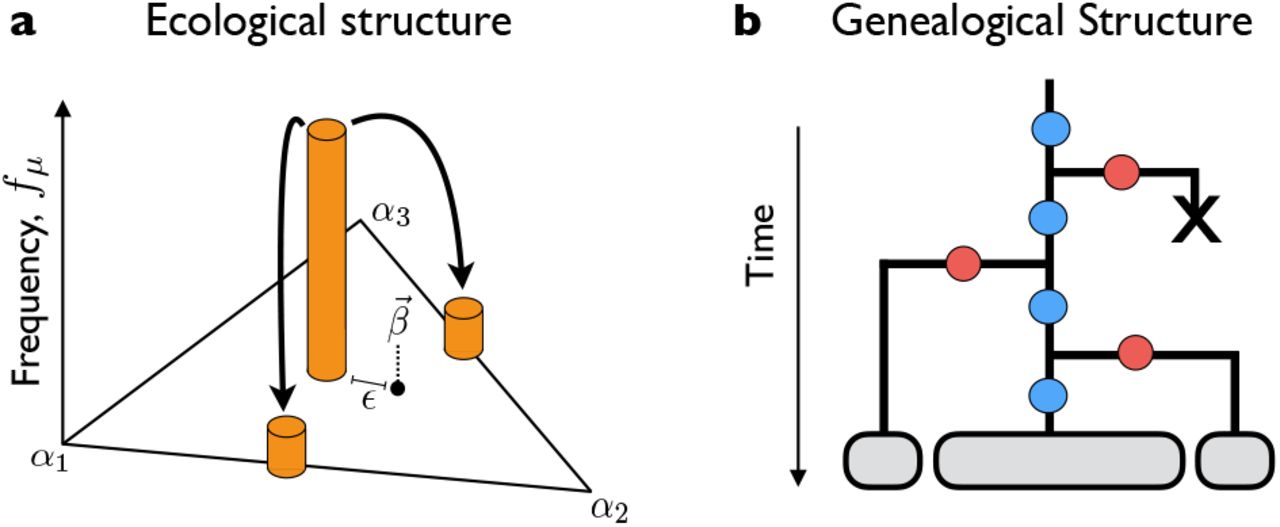
An analogous version of Fig. S2 comparing specialist and generalist initial conditions for  .
.
REFERENCES
- [1].↵
- [2].↵
- [3].↵
- [4].↵
- [5].↵
- [6].↵
- [7].↵
- [8].↵
- [9].↵
- [10].↵
- [11].↵
- [12].↵
- [13].↵
- [14].↵
- [15].↵
- [16].↵
- [17].↵
- [18].↵
- [19].↵
- [20].↵
- [21].↵
- [22].↵
- [23].↵
- [24].↵
- [25].↵
- [26].↵
- [27].↵
- [28].↵
- [29].↵
- [30].↵
- [31].↵
- [32].↵
- [33].↵
- [34].↵
- [35].↵
- [36].↵
- [37].↵
- [38].↵
- [39].↵
- [40].↵
- [41].↵
- [42].↵
- [43].↵
- [44].↵
- [45].↵
- [46].↵
- [47].↵
- [48].↵
- [49].↵
- [50].↵
- [51].↵
- [52].↵
- [53].↵
- [54].↵
- [55].↵
- [56].↵
- [57].↵


