

Abstract

Epigraph: The Naming of Euplotid “The cell is a system that is capable of creating and conserving its own code” --Marcello Barbieri[1]
The Cambrian explosion is responsible for the cementing of animal life on this planet; phylogenetic analysis appears to indicate that all metazoans originated from a single common flagellated organism, something resembling a Euplotid. Darwin has noted that this event does not seem to follow with a traditional evolutionary view, the speed and emergence of metazoans accelerated orders of magnitude when compared to the life that preceded them. There have been many attempts to explain this event, from Oxygen concentration to complexity thresholds, but no-one has considered that clues may lie within the genetic code itself, after all, this code is fundamental for the evolution of life as we know it.
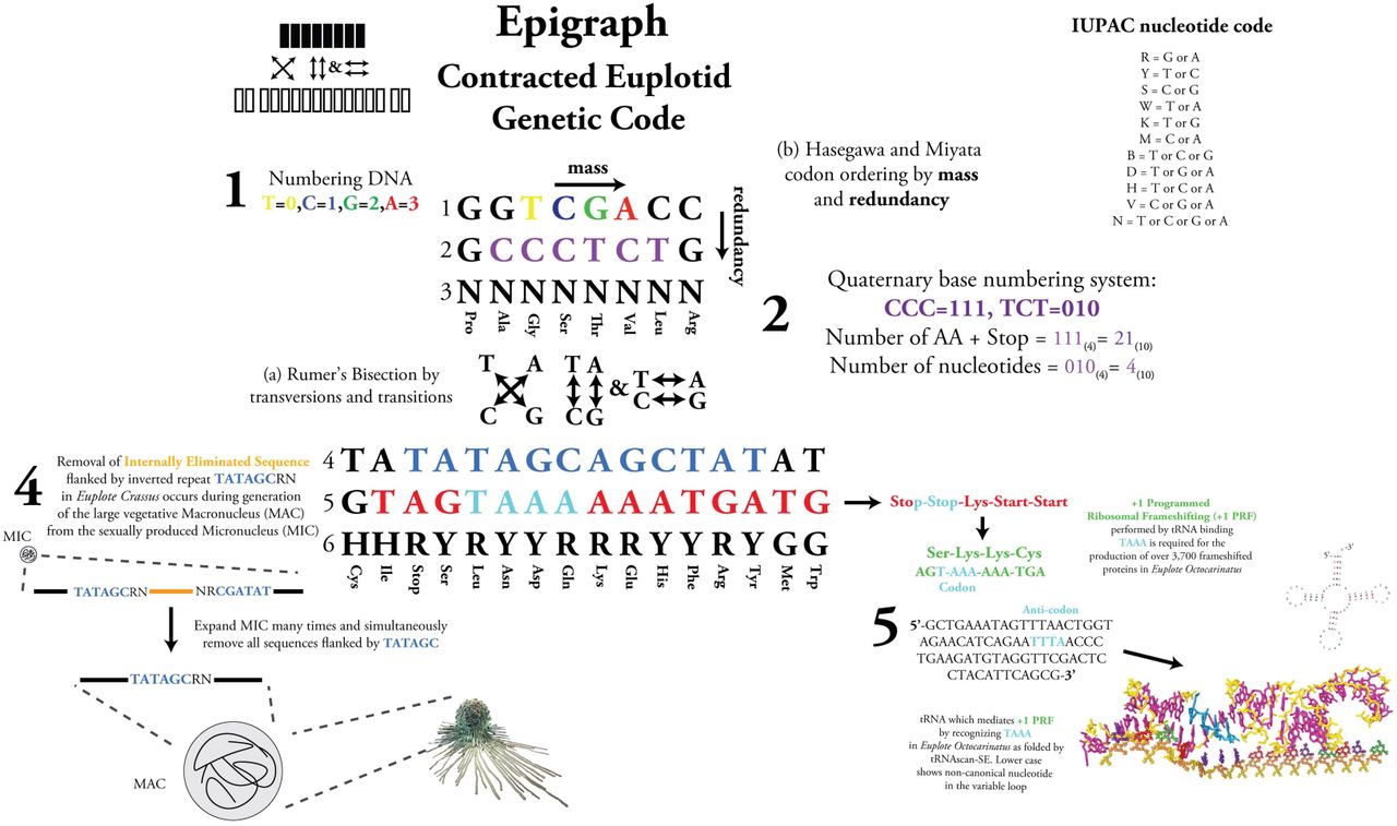
A number of patterns have been observed within the codons, but a particularly interesting combination of two rules allows for the writing of the Euplotid genetic code in a contracted manner. By combining Rumer’s Bisection (a)[2] with Hisagawa-Minata’s[3] ordering by codon redundancy/mass (b) and applying them to the Euplotid genetic code we are able to contract and arrange the codons as first shown in Makukov et al[4].
Makukov et al discovered the protacted Euplotid codon arrangement and go well into the arithmetic interpretation, that is to say the part dealing with arithmatic. Below is an ideographical interpretation:

Contracted codons of the Euplotid Genetic code
GGTCGACC: How to number DNA, 0=T, C=1, G=2, A=3
GCCCTCTG: What radix number system to use. CCC = 111 (base 4) = 21 (base 10) = number of amino acids + stop codon. TCT = 010 (base 4) = 4 (base 10) = number of nucleotides.
NNNNNNNN: Is able to complement “GGTCGACC”
TATATAGCAGCTATAT: Euplotids remove Internal Eliminated Sequences (IESs) in the process of generating the large vegetative Macronucleus (MAC) from the small sexually produced Micronu-cleus (MIC). The Euplote Crassus consensus sequence is 5′-TATrGCRN-3′[5].
GTAGTAAAAAATGATG: Translating from left to right starting w/ TAG would produce: Stop-Stop-Lys-Start-Start using the canonical genetic code, but in Euplotids +1 Programmed Ribosomal Frameshifting (+1 PRF) occurs at AAA sites preceding stop codons due to a tRNA recognizing UAAA instead of UAA[6] [7]. So if we perform a +1 PRF and read starting at AGT we get: Ser-Lys-Lys-Cys (brief movie showing the process). This is only in Euplotids due to TGA coding for Cys instead of stop. +1 PRF in Euplotids is used to generate functional proteins from fusing different reading frames in over 3,700 proteins, including the Reverse Transcriptase of LINE-elements, ORF2 [8]
HHRYRYYRRRYYRYGG: Is able to complement “TATATAGCAGCTATAT”
Due to this unique genetic signature, I decided to name this quantized geometric model of the eukaryotic cell, “Euplotid”.
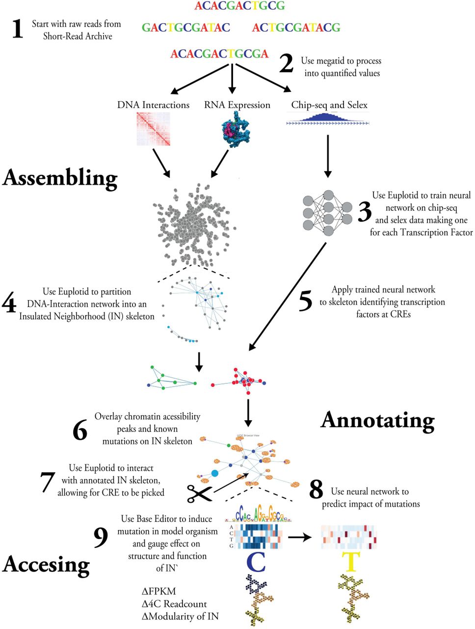
2.0.2 Introduction to Euplotid’s playground Life as we know it has continued to shock and amaze us, consistently reminding us that truth is far stranger than fiction. Euplotid is a quantized geometric model of the eukaryotic cell, a first attempt at quantifying, using planck’s constant geometric shape as its base, the incredible complexity that gives rise to a living cell. By beginning from the very bottom we are able to build the pieces, which when hierarchically and combinatorially combined, produce the emergent complex behavior that even a single celled organism can show. Euplotid is composed of a set of quantized geometric 3D building blocks and constantly evolving bioinformatic pipelines encapsulated and running in Docker containers enabling a user to build and annotate the local regulatory structure of every gene starting from raw sequencing reads of DNA-interactions, chromatin accessibility, and RNA-sequencing. Reads are quantified using the latest computational tools and the results are normalized, quality-checked, and stored. The local regulatory neighborhood of each gene is built using a Louvain based graph partitioning algorithm parameterized by the chromatin extrusion model and CTCF-CTCF interactions. Cis-Regulatory Elements are defined using chromatin accessibility peaks which are then mapped to Transcription Start Sites based on inclusion within the same neighborhood. Deep Neural Networks are trained in order to provide a statistical model mimicking transcription factor binding, giving the ability to identify all Transcription Factors within a given chromatin accessibility peak. By in-silico mutating and re-applying the neural network we are able to gauge the impact of a transition mutation on the binding of any transcription factor. The annotated output can be visualized in a variety of 1D, 2D, 3D and 4D ways overlaid with existing bodies of knowledge, such as GWAS results or PDB structures. Once a particular CRE of interest has been identified by a biologist the difficulty of a Base Editor mediated transition mutation can be quantitatively observed and induced in a model organism.
Detailed Abstract
3. Introduction

Introduction to the quantized 3D building blocks organizing the genome: Going from the bottom up and using planck’s quanta as a basic building block we are able to create the 3D building blocks which comprise a eukaryotic cell. Using our current understanding of the organization of the genome we are able to create a pseudo physical model, a brief video goes through the figure as a whole: full introduction video
The physical hierarchy of the genome begins with the smallest and most simple building block, planck’s constant, a quanta. The debate as to what geometric shapes define our 3D reality harps back to at least 360 B.C. when the philosophy behind the physicality of elements was established[9] as exemplified in the Platonic Solids. In Timeus some of the philosophical groundwork was laid for the understanding that compounds were made up of space-filling elements, and that through their combination one could create new compounds with very different properties than the sum of their parts. In the early 1800s the first atomic model was developed, able to explain chemical reactions as physical rearrangement of indivisible atoms[10]. The indivisibility of this atom was challenged in 1897 when the electron was discovered; the so called “plum pudding” model was born[11]. The plum pudding lasted until 1911 when the infamous gold foil experiment proved that the positively charged “pudding” was actually a nucleus[12]. This nucleus contained protons, and later, was found to contain neutrons as well. Although the presence of the electron can be measured all around the positively charged nucleus they appear to be present at higher likelihoods in certain locations. During the 1930s a quantum electro dynamic model was born which is able to predict the probability of observing electrons at specific locations at unparalleled accuracy[13]. In tandem, particle physics gave us a clearer picture of the nucleus, as a tightly packed ball of protons and neutrons, each made up of quarks. This left us with the atom as a tightly packed nucleus surrounded by a field of electron “probability”, doomed to never truly ever know exactly what will happen. In 2012 an interesting proposition was put forth, what if a quanta of energy itself had a physical shape, albeit 2D?[14] This gave rise to a novel way of interpreting all the previously developed theories, and coincidentally, loops back to Plato’s first Platonic solid, the tetrahedron.
Around 1860 the philosophy was developed in order to explain the natural evolution which gave rise to the diversity in organisms as seen today[15]. The concept that all organisms come from a single common ancestor is in some ways disturbing in its simplicity, but is a key insight in order to understand our world as a whole. At the same time the physical explanation behind the tree of life was being laid down through the use P. Sativum[16]. The understanding that traits are inherited was extended to human disease in 1908 through the study of alkaptonuria[17]. Although the mechanism of inheritance was established, the physical material encoding the instructions for these traits was still hotly debated, was it proteins or nucleotides? The debate was settled in the 1930s through the use Pneumococcus and its virulence as a phenotypic trait[18]. With the chemical composition of the transforming material settled as nucleotides, the code defining the transition from DNA to RNA and then Amino Acids was solved during the 1950s[19]. The genetic code which governs how an organism moves information between DNA, RNA, and Amino Acids appears to be pliable, and novel mechanisms continue to be found. Although we had found the chemical composition of the information storing component, we knew almost nothing as to how DNA’s shape was used to encode information. Two rules were discovered during the 1950s which began to decode DNA, Chargaff’s rules. The first rule laid the groundwork for the structure of DNA to be solved, that is to say %C=%G and %A=%T[20]. DNA’s structure was famously solved in 1953, giving a physical explanation to Chargaff’s first rule and a major step in the physical organization of the genome was solved, the 3D shape of an oligonucleotide[21]. It is very interesting to note that although a physical explanation was found for Chargaff’s first rule, his second remains unexplained.
Our understanding of the physical hierarchy of the genome was questioned when it was discovered that the canonical nucleotides existed within DNA in edited forms. The first conclusive proof of Cytosine Methylation on the 5th Carbon (5mC) was published in 1980 [22]. In the following years a number of other modified states were found for Cytosine, including: 5-hydroxylmethylcytsine (5-hmC), 5-formylcytosine (5-fC) and 5-carboxylcytosine (5-caC), while the enzymes mediating them were found and characterized: TET, DNMT and AID[23].
The first amino acid was discovered in 1806, asparagine. Over the next decade the rest of the canonical 20 amino acids were discovered, isolated, and their properties carefully measured[24]. The amino acids form the functional unit of peptides, which when strung together and folded, create proteins. Our understanding of how these mechanical subunits come together is still in its infancy, in much due to our misunderstanding of the charge and mechanics at the most fundamental level. With a sharply defined boundary between energy and matter we are able to model interactions between these small protein building blocks in a far more natural, newtonian manner, while mantaining quantum accuracy.
Much of the confusion between the carrier of genetic information was due to DNA’s extremely tight association with positively charged protein complexes called the nucleosomes[25]. The nucleosome’s components and structures were developed and refined through the 1940s and 50s, with the core nucleosome’s structure and components resolved at near atomic resolution. Although the predominant components were solved, new variants of the nucleosome complex were discovered, and continue to be, such as the newly characterized MacroH2A variants[26]. In the 1960s post-translational modifications of the nucleosome’s tail were discovered to affect its association with DNA through changing lysine’s charge and shape[27]. This level of the genome’s physical organization allows for about 200bp to be neatly packaged, tagged and accessed, laying the groundwork for larger diameter fibers.
Chromatin can be understood as any shape of DNA that has a diameter larger than the canonical 10nm beads on a string nucleosome model. The exact shape and the in-vivo existence of the 30nm chromatin fiber has been hotly debated. It appears that there exists evidence for both sides, and in reality, it seems likely that the chromatin is a dynamic fiber, capable of deforming, memorizing, and reacting[28]. Within the last decade we have begun to probe how the shape and regulation of this fiber can impact its shape and function, namely we have just begun to unravel the consequences of histone tail marks on the conformation of chromatin. Seemingly, chromatin is much more than the sum of its parts, and a key way of maintaining information in the shape of our genome[29].

The local regulatory structure of Eukaryotic genes is largely maintained by clever use of CTCF and Cohesin whose misregulation can lead to disease
Once we had conclusively settled on DNA as the transforming material we could begin to elucidate the set of ordered reactions which takes DNA and decodes it to amino acids through an RNA intermediate. Throughout the 1970s the first steps of RNA-Polymerase mediated transcription were solved and the key players identified[30]. It was quickly discovered that not all RNA is destined for translation, only the subset coined “messenger RNA” or mRNA. RNA-Pol II was shown to be the holoenzyme responsible for the polymerization of this mRNA, which is in the reverse complement of the DNA template. As the constituents discovered for the pre-initiation complex (PIC) grew during the 1980s, it was found to form around the canonical TATA DNA motif, coined the “TATA-box”[31]. This TATA box has a specific 3D shape which causes a bend of the DNA at approximately 80 degrees when bound by proteins called Transcription Factors (TFs). The Mediator protein “arm” complex is attached to this TATA DNA bend. Mediator, aided by Nipbl, allows for the threading of this bent DNA through a small protenaicous band structure known as Cohesin, thereby creating a small loop[32]. The elongation of RNA-Pol II is preceded by TFIIH mediated phosphorylation of the C-Terminal Domain (CTD) of RNA-Pol II [33]. How the phosphorylation of the CTD impacts its interaction with the extremely electronegative surface of RNA-PolII has not been studied at the quantum level.

Chromatin extrusion allows for the stacking of Cohesin rings on CTCF
Recently it was found that the natural motor motion of RNA-Pol II during elongation serves to push this Cohesin ring, causing it to extrude a loop, bringing seemingly distant parts of the genome into direct physical proximity. This extrusion process continues until a bound CCCTC-Binding Factor (CTCF) is encountered, stopping the progression of Cohesin and causing the ring to stack at that bound CTCF site. CTCF’s history in research took many turns, being assigned a plethora of roles, from enhancer to repressor, until its eventual establishment as a looping factor[34]. The rate of release of Cohesin at CTCF sites is also actively controlled by acetylation of the ring, while CTCF’s binding can be impacted by the methylation of its DNA binding motif[35]. The intricate details are still debated, but overall it appears that the clever regulation of on/off rates on DNA for these three pieces, CTCF, Cohesin, and RNA-Pol II, allows for the creation of dynamic structures capable of reacting to differing cellular states, tuning a gene’s local regulatory structure to adapt to specific environments. Although a CRE is able to influence the expression of any gene in extreme genomic proximity, the larger structures encompassing the CRE can cause it to impact TSSs from seemingly distant promoters[36]. The local regulatory structure of Eukaryotic genes is dependent on their own expression through the extrusion of Cohesin rings, this intriguingly forms a sort of feedback mechanism. The speed and dynamics of this transcriptional feedback mechanism may be influenced by certain charge dynamics from localized areas of Acetylation, such as those mediated by the H4 HAT complex or the asymmetrically loaded Acetylation of H3 at Super Enhancers[37]. Although these effects originate down from the very basic levels of the physical hierarchy, when aggregated together, it may be possible that they impact larger dynamics. We are beginning to see modeling approaches reaching the scales necessary to tackle chromatin looping questions, these models will continue to develop and gain in accuracy and generality. The physical hierarchy that controls the relation between CREs and their respective TSSs is a complex and extremely fine tuned process, but it may be that this complexity originates from very simple building blocks.

The definition of the local regulatory neighborhoods of genes is limited by linear thinking and genomewide measures
The regulation of transcription through the looping of CREs and TSSs appears to be often perturbed by disease causing mutations, especially those which are associated with non-coding CREs[38]. By combining recently developed methodologies to probe RNA-Seq, DNA-DNA interactions and Chromatin Accessibility with our recently acquired knowledge of the physical hierarchy governing the folding of the genome, we are able to build a rough quantized picture of the 3D regulatory landscape of the genome. In order to digest this information in a manner which can guide experimentalists it is key to annotate and allow for easy access of these structures. Taking advantage of a number of recent developments in unrelated fields we are able to do just that; we provide a constantly evolving platform capable of allowing biologists to make physically informed decisions as what variation is causing the phenotype based on quantumly accurate models, virtually anywhere, anytime.

Euplotid solution
4. Results
4.1 Assembling

Assembling the local regulatory structure of genes
Determining the right local regulatory structure of a gene can be easy by eye but defining and performing this task computationally is very difficult.
4.1.1 Define Graphs
We begin with set of Nodes, defined as a DNA range, with a left and right boundary, for example: chr16:55155024-53806737. We then add a set of Edges, defined as DNA-DNA interactions, or loops. These loops can be recovered from living cells using a variety of methods, such as Hi-C, In-situ Hi-C, ChiA-PET, HiChIP, GAM, etc, each having their own wet and dry processing protocol, with all dry implemented within Megatid.
4.1.2 Define starting nodes
The initial starting conditions are when every Node is its own unique IN of size 1. We can use RNA-seq as a poor-man’s proxy for the rate of Cohesin-RNAPolII mediated chromatin extrusion. The processing of raw RNA-Seq reads can be quickly performed within Megatid using STAR to align the reads and RSEM to quantify RPKM[39] [40]. We begin the algorithm by sorting the starting nodes by RPKM.
4.1.3 Crawl outward adding nodes
Beginning at each highly transcribed Transcription Start Site we select the neighbor which would increase the overall network architecture the most as defined by Modularity and reassign its IN if the entire IN is encompassed within a single CTCF-CTCF interaction[41–43].
4.1.4 Reach modularity equlibrium
Continue checking for valid reassignments until no more moves exist which increase the overall graph’s modularity, thereby reaching an equilibrium.
4.1.5 Recover rough X,Y,Z location of IN
Take all DNA-DNA interactions and combined with Lamin A/B1 Chip-Seq estimate the rough nuclear X,Y,Z position of each IN node by feeding the data through HSA[44]. The size of the node is defined using the sum of all reads falling within chromatin accessible regions.
4.2 Annotating

Annotating the Insulated Neighborhoods
4.2.1 Color nodes
After assembling the Insulated Neighborhood skeleton it is key to be able to visualize the impact of Histone modifications on the local regulatory structure, therefore we simply color the nodes of the genomic graph by histone modifications in the given cell state of interest. Specifically, Red if node overlaps only with H3K27Ac and blue if it overlaps H3k4me3 [45].
4.2.2 Train neural networks
Begin by training Convolutional Neural Networks (CNNs) based on all chip-seq and SELEX data for all TFs ever surveyed. The initial implementation of Euplotid uses pre-trained CNNs from Deepbind[46]. These CNNs are able to identify the TFs which fall under each chromatin accessiblity peak, but in order to understand the peak as a whole Euplotid takes advantage of Basset to train neural networks which are capable of predicting changes in chromatin accessibility[47]. Basset is trained on all available chromatin accessibility data in ENCODE, DNAse of 180 different cell lines. Basset is therefore able to perform in-silico simulations to gauge the impact of a given mutation on the the complex as a whole (SNP Accessibility Difference (SAD) profile), by combining this with the CNNs from Deepbind, we are able to make a prediction as to what factor is causing this change.
4.2.3 Select chromatin accessibility peaks
Taking all chromatin accessibility peaks within a set distance (50kb) from all the nodes of a given IN allows us to identify the relevant areas of chromatin which are actively being used in this particular cell state, some potentially acting as Cis-Regulatory Elements. Any method of chromatin accessibility is appropriate, DNAse-seq, ATAC-seq, MNAse-seq, etc, all can be used as inputs.
4.2.4 Identify TF constituents
Applying the trained neural network on each chromatin accessibility peak we are able to identify the constiuents, thereby identifying complexes putatively making up each Cis-Regulatory element. Currently this is performed by Deepbind, but a custom built pytorch based network will soon be implemented[48].
4.2.5 Select and annotate SNPs/CNVs
We can then include all SNPs/CNVs within dbSNP which overlap the chromatin accessibility peaks within the IN[49]. This variation is then annotated with the following data if available: eQTL in 32 tissues (FastQTL+GTeX), ease of CRISPR editing (GT-Scan2), results of over 2,000 GWAS studies (GRASP), 667 Methylomes (NGSMethDB), estimate of deleteriousness (CADD Score)
4.2.6 Predict effect of SNPs/CNVs
For each variant which falls within the IN we perform an in-silico mutational analysis. This in-silico mutational analysis is simple, predict the chromatin accessibility with and without the variant. The difference in SNP accessibility (SAD score) is calculated by Basset with the pre-trained networks as described above.
4.3 Accessing

Accessing the Insulated Neighborhoods
Visualization of large graphical structures with huge amounts of data which are navigable in a stable easy to deploy environment has been a huge barrier. Docker, Python, Resin, Plotly and Jupyter together allow for deployment, visualization, and interactivity across all computing architectures[50] [51] [52] [53]. The entire analysis can be replicated and edited in front of your eyes, creating unprecedented trans-parency between input data and output analysis. You can use Euplotid to make mechanistic predictions from any device, in any web browser, running on virtually anything, from almost anywhere.
4.3.1 Pick cell type and condition
Using widgets in Jupyter we are able to dynamically access the annotated local regulatory structure of every gene stored as graphs within JSONs through the backend. A Jupyter widget is a simple lightweight node.js wrapper to traditional python methods. Here we can pick what cell type and condition we want to investigate.
4.3.2 Pick annotated Insulated Neighborhood
After picking a cell type and condition the list of annotated INs will be populated. A simple dropdown sorted by name is provided.
4.3.3 UCSC genome browser view
If the user wants visualize the data in the traditional 1D manner it is possible to load the data into the UCSC genome browser. In this case we set the linear left and right boundaries as the leftmost and rightmost node within the IN currently being viewed.
4.3.4 Annotated Insulated Neighborhood
The annotated IN is positioned according to the Fruchterman-Reingold force-directed algorithm on DNA-interaction read count in order to have a more visually pleasing view. By employing 3Djs and Plotly we are able to navigate large graphical structures with relative ease. When hovering over every DNA-Interaction node the following pieces of data are shown if available: eQTL in 32 tissues (FastQTL+GTeX), ease of CRISPR editing (GT-Scan2), results of over 2,000 GWAS studies (GRASP), 667 Methylomes (NGSMethDB), estimate of deleteriousness (CADD Score), and CNN prediction of TF identity
4.3.5 DNA-DNA interaction heatmap view
Awesome tile-based viewing tool for DNA-DNA interaction data[54]. Employing D3.js to query a robust backend, this dockerized application is able to serve huge compressed multi-resolution 2D Hi-C data essentially instantly. The compression and raw interaction handling is done by Cooler.
4.3.6 SNP accessibility difference prediction
Employing CNNs previously trained on Chip-Seq and SELEX data and combining them with LSTM networks we are able to predict the chromatin accessibility of a particular sequence in a given cell type. Taking all SNPs/CNVs which fall within the IN we then predict the impact of each of those on the accessibility of chromatin.
4.3.7 Global view
Using the X,Y,Z coordinates previously generated for each IN using HSA we are able to have a small “mini-map” corresponding to a global view of the entire nucleus. Each IN node is colored according to chromsome and the INs are connected according to genomic coordinate.
4.3.8 In-silico mutational analysis
Using previously trained neural networks we are able to view the predicted image for a given in-silico mutatation. This gives a quick and easy to assess view of the impact a given SNP has on a Cis-Regulatory element, potentially affecting its function.
4.3.9 Virtual reality view
Taking advantage of Virtual Reality (VR) technology developed for both the military and consumer markets we are able to render the annotated INs in full immersive VR. We use Unreal Engine to design, build, and deploy the VR view[55]. Tested with the HTC Vive allowing for fully immersive room-scale exploration of large complex annotated INs. A more detailed explanation is available below: Introduction to Euplotid’s playground
4.3.10 Deployment of Euplotid
INSTALL DOCKER HERE Then open your terminal or cmd and: ∼ docker run --name euplotid -p 8890:8890 -tid
-v “/your/input/directory:/input_dir”
-v “/your/temporary/directory/:/tmp_dir”
-v “/your/output/directory/:/output_dir”
-v “/your/annotation/directory/:/annotation_dir” dborgesr/euplotid:euplotid ∼
4.3.11 Try it out!
5. Discussion

Next steps and impact
Euplotid is a quantized geometric model of the eukaryotic cell that is built to evolve over time, to shed pieces and gain new ones as more powerful bioinformatic tools are created. Due to its modularity and deployability Euplotid can be used almost anywhere. Combined with emerging “Edge” computing and sequencing infrastructures such as NVIDIA’s Jetson and Oxford Nanopore’s MinION[56] the potential for on-site building and visualization, from raw sequencing data to annotated immersive VR would be possible. A strategy which may be limited in immediate computing power but is able to deal with privacy concerns from the ground up.
In the future it will be possible to combine multiple images of Euplotid running in tandem mimicking tissues, with each Euplotid image communicating between each other and being slightly different, incorporating single-celled resolution techniques. Due to Euplotid’s foundational principles we are able to capture movement and mechanics down to the quantum level but remain extremely efficient and tractable, we render what we need to look at. The availability and ease of use will allow Euplotid to spread around the globe with relative ease.
7 Methods
The process of building Euplotid began with taking raw sequencing reads stored in a few different formats and processing it all the way to quantified values. Due to the pliability, breadth, and flexibility of the methods they will be documented within their own Jupyter notebook. Acting as both the documentation and the pipeline itself this format allows for seamless data integration.
Hello world intro to programming and Jupyter’s capabilities helloWorld O*.
Databases and good tools to crawl the internet for interesting datasets and hypothesis databases-Tools O*.
Fetch any type of sequencing data from SRA getFastqReads O
QC, trim, and filter sequencing reads fq2preppedReads O
Call peaks from Chip-Seq and Chromatin Accessibility reads fq2peaks O
Call normalized interactions from ChiA-PET reads fq2ChIAInts O
Call normalized Interactions from HiC reads fq2HiCInts O
Call normalized interactions from Hi-ChIP reads fq2HiChIPInts O
Call normalized interactions from DNAse-HiC reads fq2DNAseHiCInts O
Call normalized expression and counts from RNA-Seq reads fq2countsFPKM O
Call differentially expressed genes from RNA-seq counts countsFPKM2DiffExp O
Call normalized counts, miRNA promoters, and nascent transcripts from Gro-Seq reads fq2GroRPKM O
Call normalized interactions from 4C fq24CInts O
Build, annotate and add INs to global graph for a given cell state using DNA-DNA interactions, Chromatin Accesibility, and FPKM addINs *
View current built and annotated INs for all cell types viewINs O*.
Search for and/or manipulate annotation and other data available to euplotid annotationManage-ment O*.
Description of default software packages and images installed, how to get new ones, and which ones are currently installed. packageManagement O*.
Find clusters of interconnected nodes (Communities) using a Louvain algorithm then visualize the results vanillaCommunities
Create, manipulate, and visualize cool DNA-DNA interaction files chilledInteractions
Design Base Editor and sgRNA plasmids for transition mutation at picked Cis-Regulatory Element CRE2plasmid
[O] = Megatid compatible [*] = Euplotid compatible [.] = Minitid compatible
7.1 helloWorld
Hello world intro to programming, ipython, and Euplotid
7.2 databasesTools
Databases and good tools to crawl the internet for interesting datasets and hypothesis. Some examples include GTeX, uniprot, SRA, GEO, etc, check them out!!
7.3 getFastqReads
Allows you to use Tony to find local fastq.gz files OR provide an SRA number to pull from
7.4 fq2preppedReads
Take fq.gz reads and QC them using FastQC checking for over-represented sequences potentially indicating adapter contamination. Then use cutadapt and sickle to filter and remove adapters. Can also use trimmomatic for flexible trimming.
7.5 fq2peaks
Take fq.gz align it using bowtie2 to the genome. Then using Homer software pick the type of peak (histone, chip-seq, dnase, etc) and chug through to get bed files of peaks. Can also use MACS2 w/ specific analysis parameters to deal with different types of peak finding problems.
7.6 fq2ChIAInts
Take fq.gz reads, prep them by removing bridge adapters (can deal with either bridges), align, find interactions, normalize, and spit into cooler format for later viewing. Can perform analysis using either Origami or ChiA-PET2
7.7 fq2HiCInts
Take fq.gz reads and chug them through HiCPro w/ tuned relevant parameters. In the end spits out a cooler file which can be loaded for further visualization.
7.8 fq2HiChIPInts
Take fq.gz reads and chug them through customized Origami pipeline and customized HiCPro pipeline. In the end spits out a cooler file which can be loaded for further visualization.
7.9 fq2DNAseHiCInts
Take fq.gz reads and chug them through HiCPro pipeline. In the end spits out a cooler file which can be loaded for further visualization.
7.10 fq2countsFPKM
Take fq.gz reads and chug them through STAR aligner and then RSEM pipeline. In the end spits out a counts vs transcripts matrix and a normalized transcript/gene FPKM matrix.
7.11 countsFPKM2DiffExp
Take RNA-seq count and FPKM matrix and run any one of many R packages (DE-Seq2,DESeq,EBSeq,edgeR…) to call differentially expressed genes. Plotting and interactive visualization of results included
7.12 fq2GroRPKM
Take fq.gz reads and align them using bowtie2 then find nascent transcripts using FStitch and miRNA promoters using mirSTP
7.13 fq24CInts
Take fq.gz reads and align them using bowtie2. Chug them through HiCPro and/or custom pipeline to get cooler file
7.14 addINs
Build, annotate and add INs to global graph for a given cell state using DNA-DNA interactions, Chro-matin Accesibility, and FPKM.
7.15 viewINs
View current built and annotated INs for all cell types
7.16 annotationManagement
Search for and/or manipulate annotation and other data available to euplotid
7.17 packageManagement
Description of default image and the software packages that are installed, also how to get new packages, and how to export environment in yaml file for others to replicate analysis.
7.18 vanillaCommunities
Find clusters of interconnected nodes (Communities) using a Louvain algorithm then visualize the results
7.19 chilledInteractions
Create, manipulate, and visualize cool DNA-DNA interaction files
7.20 CRE2plasmid
Design Base Editor and sgRNA plasmids for transition mutation at picked Cis-Regulatory Element
6 Acknowledgements
I thank the Rick Young lab for many productive and informative discussions and help with flow of writing.
8 References
- [1].↵
- [2].↵
- [3].↵
- [4].↵
- [5].↵
- [6].↵
- [7].↵
- [8].↵
- [9].↵
- [10].↵
- [11].↵
- [12].↵
- [13].↵
- [14].↵
- [15].↵
- [16].↵
- [17].↵
- [18].↵
- [19].↵
- [20].↵
- [21].↵
- [22].↵
- [23].↵
- [24].↵
- [25].↵
- [26].↵
- [27].↵
- [28].↵
- [29].↵
- [30].↵
- [31].↵
- [32].↵
- [33].↵
- [34].↵
- [35].↵
- [36].↵
- [37].↵
- [38].↵
- [39].↵
- [40].↵
- [41].↵
- [42].
- [43].↵
- [44].↵
- [45].↵
- [46].↵
- [47].↵
- [48].↵
- [49].↵
- [50].↵
- [51].↵
- [52].↵
- [53].↵
- [54].↵
- [55].↵
- [56].↵


