

Abstract
Recent studies have established that the circadian clock influences onset, progression and therapeutic outcomes in a number of diseases including heart disease and cancer. There are, however, no tools to monitor the functional state of the circadian clock and its downstream targets in humans. We provide such a tool and demonstrate its clinical relevance by an application to breast cancer where we find a strong link between overall survival and our measure of clock dysfunction. We use a machine-learning approach and construct an algorithm called TimeTeller which uses the multi-dimensional state of the genes in a transcriptomics analysis of a single biological sample to assess the level of circadian clock dysfunction. We demonstrate how this can distinguish differences between healthy and diseased tissue and demonstrate that the clock dysfunction metric is a potentially new prognostic and predictive breast cancer biomarker that is independent of the main established prognostic factors.
Introduction
The cell-endogenous circadian clock regulates tissue-specific gene expression in cells that drives rhythmic daily variation in metabolic, endocrine, and behavioural functions. Indeed, around half of all mammalian genes are expressed with a 24-hour rhythm (1, 2). Moreover, recent studies demonstrated that the circadian clock influences therapeutic outcomes in a number of diseases including heart disease and cancer (3–9), and that disruption of the normal circadian rhythm and sleep (e.g. through shift work) is associated with higher risk of obesity, hypertension, diabetes, CHD, stroke and cancer (10–13).
A principal aim of circadian medicine (14, 15) is to develop techniques and methods to integrate the relevance of biological time into clinical practice. However, although circadian disruption is known to affect multiple organs, it is difficult to monitor the functional state of the circadian clock and its downstream targets in humans. Consequently, there is a critical need for tools to do this that are practical in a clinical context. Our focus is on the development of such a technique, and here we will illustrate its utility to predict breast cancer survival. We present a machine-learning approach to measuring circadian clock functionality from the expression levels of 10-15 key genes in a single tissue sample. Our algorithm is applied to breast cancer where previous studies have highlighted the relevance of circadian clocks for carcinogenesis and treatment effects (16–19) but where no simple method would currently allow its measurement in daily oncology practice. We find a strong link between overall survival and our measure of clock dysfunction.
There are now several algorithms which aim to estimate the time at which a transcriptomic dataset was collected using the expression levels of the core clock genes (14, 20–25). While these have hinted at the idea of using such a time-telling approach to measure circadian clock functionality (23) they are not purposely constructed to do this, but rather to predict internal timing of functional host circadian systems (Note S6). Moreover, for practical use, it is highly desirable to be able to do this using just a single clinical sample, and these algorithms do not attempt this. We therefore developed a new algorithm called TimeTeller to estimate clock functionality from a single sample.
While in the cells of most healthy tissues the cell cycle is gated or phase-locked by the circadian clock (26, 27), cancer cells often escape this control and display altered molecular clocks (28–30). Dysregulation of clock genes promotes tumorigenesis (22) through mechanisms involving the cell cycle (31, 32), DNA damage (33), and metabolism (34). Moreover, the circadian clock rhythmically controls many molecular pathways which are responsible for large time-of-day dependent changes in drug toxicity and efficacy (3, 4, 35). It is therefore of interest to determine whether the functionality of the clock in tumour tissue is a prognostic factor for treatment response and survival.
We demonstrate that TimeTeller can characterise differences in the distribution of the dysfunction metric between healthy and diseased tissue and between different disease strata, and that the dysfunction metric can be used as a prognostic factor to identify differences in outcome. In particular, we show that in a large cohort of patients with non-metastatic breast cancer the resulting TimeTeller dysfunction metric is a prognostic factor for survival and provide evidence that it is independent of other known factors. In this cohort, 82% of the patients with good clock function (i.e. for which the dysfunction metric is below a natural threshold) survive past ten years while only 62% of the others survive as long.
Our approach directly assesses the systemic functionality of a key regulatory system, the circadian clock, from one sample. A key aspect is that we directly assess the multi-dimensional state of the clock genes and study the coordinated behaviour of all the genes together rather than focus on each gene separately. In this way, we can measure the functionality of the clock system as a whole much more effectively.
Results
The mouse and human versions of TimeTeller are trained on two different datasets. The mouse dataset, from Zhang et al. ((1), Note S1) consists of the transcriptomes of 12 mouse tissues measured every 2 hours over 48 hours while the human training data set from Bjarnason et al. ((36), Note S1) comes from punch biopsies of oral mucosa taken every four hours over 24 hours from five females and five males. This human dataset was chosen because a key initial aim was to develop TimeTeller in order to analyse clock function in the tumour biopsies from the REMAGUS trial (37) and our analysis suggested that it was important to match the microarray technologies (Fig. S2) which in this case was Affymetrix U133 2.0. The procedure for using these datasets to successfully produce TimeTeller’s probability model is explained in the Materials and Methods section.
Rhythmicity and synchronicity analysis was used to determine the panel of genes for TimeTeller (Materials and Methods, SI Fig. S1, Table S2). This analysis is essential to ensure the choice of a panel of genes with good circadian rhythmicity combined with minimal variation across tissues and datasets. It typically produces a panel of between 10 and 16 gene probes and, for the human dataset, the genes selected were all core clock genes or key clock-controlled genes, including ARNTL (BMAL1), NPAS2, PER1, PER2, PER3, NR1D1, NR1D2 (REV-ERBα), CIART (CHRONO), TEF and DBP.
TimeTeller works on the combined expression level of these genes and calculates a likelihood curve LX(t) which for healthy tissue should express the probability that the expression profile X was measured at time t. If this time is not known, then it is natural to estimate it as the time T at which LX(t) is maximal i.e. at the maximum likelihood estimate (MLE) (Materials and Methods). Then we can characterise precision using ideas from statistics and information theory to obtain a quantity, which we denote by Θ, that characterises the imprecision of the estimate T (Materials and Methods). We call Θ the clock dysfunction metric based on the hypothesis that precise timekeeping implies good functionality.
We have tested this clock dysfunction metric using both simulated and real data. Simulated data were obtained by developing a stochastic version of a relatively detailed published model of the mammalian circadian clock (38) and stochastically simulating this (Note S5). This data was used to design the algorithm and to test the effectiveness of TimeTeller, for example, to determine the advantage of local approaches over a global one (Fig. S3, Tables S4 & S5), and to analyse TimeTeller’s effectiveness in detecting the efficiency of partial knockdowns of various efficiencies of the central clock gene BMAL1 (ARNTL). We found (Fig S7) that the efficiency of the knockdown was effectively recapitulated by an increase in Θ. We then applied TimeTeller to a number of mouse and human datasets.
In healthy tissue TimeTeller accurately assesses time and identifies variation in chronotype
To assess the accuracy of TimeTeller in estimating the time T of a sample and to evaluate the likelihood curves LX(t), we firstly tested it on the training datasets using a leave-one-out approach. For the Zhang et al. mouse data, we removed the tissues one at a time, constructed the probability model for TimeTeller using the expression profiles from the other tissues and then used TimeTeller to estimate the times of the transcriptomes for the removed tissue. For the human Bjarnason et al. data we carried out a similar leave-one-out approach but where an individual rather than a tissue was left out.

(A,B) Correlation plots for actual versus predicted time for (A) the Zhang et al. data ((1), Note S1) using 11 probes and 8 organs and (B) the human oral mucosa data ((39), Note S1) using a leave-one-out approach. The 5 male (M) and 5 female (F) subjects are identified with a different colour. (C,D) The likelihood functions LX(t) obtained for the samples from a representative time for the mouse (left) and human (right) datasets. The vertical lines mark the time of the sample and there is a likelihood curve for each sample. The maximum point of the likelihood functions is used to estimate the time when the sample was taken. (D). For each individual in the Bjarnason et al. data the residual (estimated time - real time) is plotted against the phase of the gene as measured by COSINOR. As explained in the text this shows that a substantial part of the error is actually due to variations in the individual sample’s chronotype rather than misestimation by TimeTeller. See Fig. S5 for similar plots for all genes in the TimeTeller panel.
The results are shown in Fig. 1 and the accuracy of the estimations is apparent (Fig. 1A,B). For the Bjarnason et al. human data the mean absolute error is 1.32h (Table S3) but analysis shows that much of this comes from chronotype variation. For example, Male15 and Female18 in Fig. 1B have consistent, yet opposite, phase shifts in their estimated times. To further understand this, we plotted the error in the TimeTeller estimate against the phase of each of the genes in the TimeTeller panel (Fig. 1D & Fig. S5), using COSINOR (40) to measure gene phase. The part of this error at a given time not due to chronotype variation is indicated by the distance of the plotted points from the line y = x + pg where pg is the expected phase of the gene at that time, shown by the horizontal black line. We see that the points are typically very close to y = x + pg and that the disposition of the points is similar across genes (Fig. 1D & Fig. S5). We are therefore able to identify coherent phase variation in the clock genes for each individual.
For the mice, no coherent phase shift was found for any of the tissues as would be expected from their genetic homogeneity and the mixing of material from multiple mice. Moreover, in this case the use of the full 48-hour space allows us to observe that TimeTeller’s transcriptomic time signature at CTt is essentially the same as at CT(t+24). This means that there is no significant change to the circadian clock gene shape after the mice have been in the dark for an extra 24 hours.
Healthy tissue clocks in mice are characterised by a clear upper threshold
The range of Θ values resulting from applying TimeTeller to the mouse training dataset using a leave-one-out approach as above are shown in the histogram in Fig. 2A. The upper bound to this range helps us to define what Θ values represent a functioning circadian clock. The majority of the data has Θ < 0.1, but the distribution has a tail up to approximately Θ = 0.2. We therefore define good clock function (GCF) for mouse samples as those having Θ < ΘGCF = 0.2. We refer to thresholds chosen in this way as a priori as they have the advantage of being chosen naturally without the potential issues associated with tuning and optimisation, for example to maximise statistical significance.
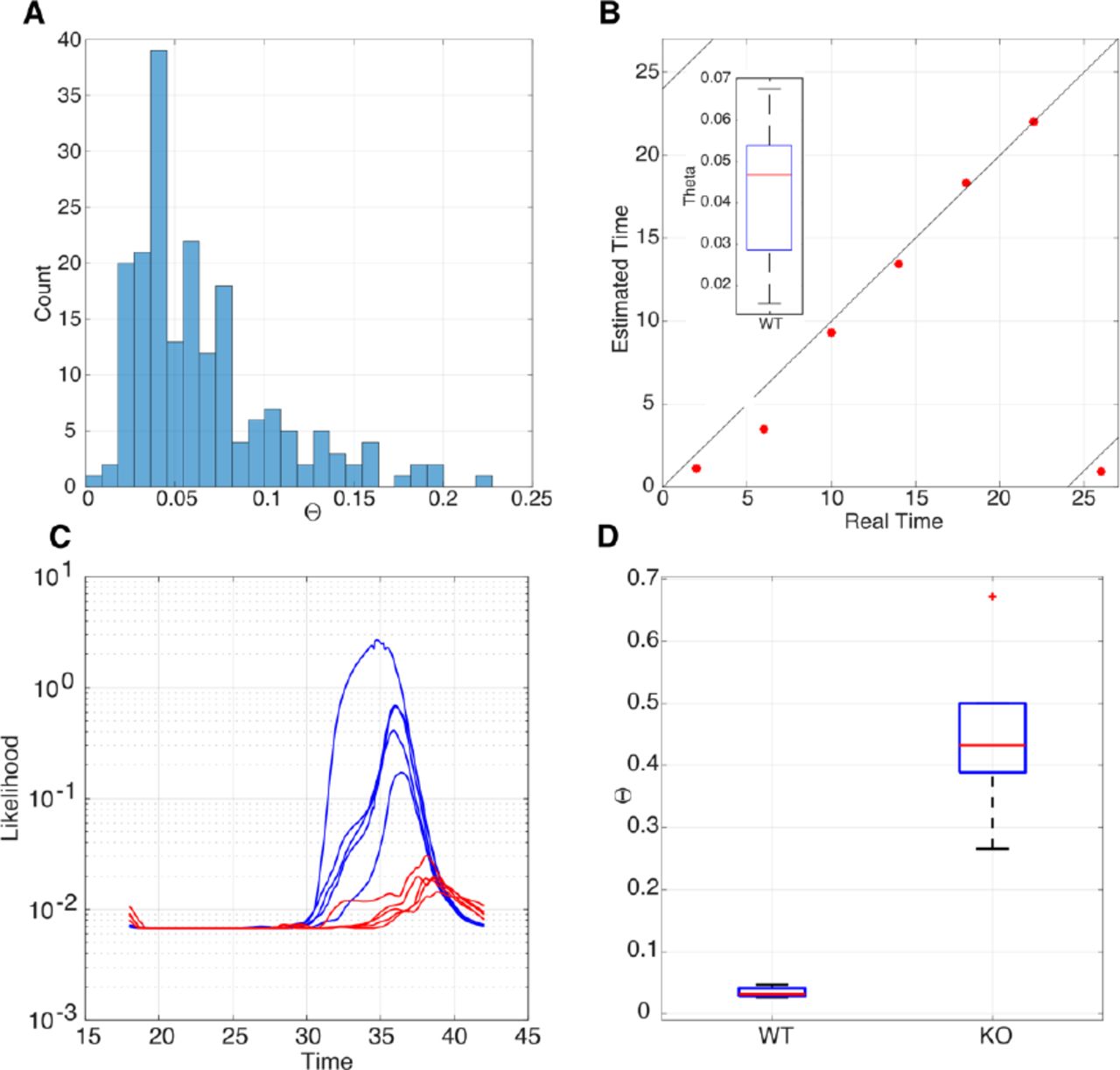
A. Histogram showing the distribution of Θ values for the Zhang et al. data. For all 182 samples of the Zhang data, the distribution of Θ values has a median around 0.05, a tail that extends to approximately 0.2 and two outliers. B. Scatter plot showing the real time versus estimated time for the LeMartelot et al. liver timecourse data together with the observed range of Θ values (inset). C. Likelihood functions for the MLE time T of samples of the Fang et al. data. They have been plotted on a logarithmic scale to reveal structure in the very low KO curves. Blue curves represent WT samples with clear peaks around CT32-36, and the negligible amplitude curves in red for the KO data. D. Box plot of Θ values for WT and KO data. There is a very significant difference between the groups. Wilcoxon’s logrank test p < 10−6.
We compared the above results with the estimation of time T and the Θ values in another published mouse dataset, Le Martelot et al. ((41), Note S1.2), which uses the same microarrays and obtained very good agreement (Fig. 2B). The mean absolute error for time estimation is less than one hour. The Θ values range between 0.02 and 0.11 with one value at Θ = 0.17 (Fig. 2B). Thus, all values fall within the GCF criterion Θ < ΘGCF defined in the previous section.
TimeTeller can identify perturbed but functioning clocks
The gene REV-ERBα is regarded as the main controller of the ZT18-24 phase of the mammalian circadian clock (42) and, interestingly, activation of clock REV-ERBα can be a therapeutic approach for several types of cancer (43) and life-threatening cholangitis (44). Thus, knocking REV-ERBα out leaves a functional but perturbed clock when compared to wild-type mice (42). Therefore, we applied TimeTeller to an experimental dataset Fang et al. (42) comparing liver samples of REV-ERBα deficient and wild type mice entrained to LD12:12 cycles. Since REV-ERBα is one of the panel of genes used in TimeTeller it would not be surprising that TimeTeller could distinguish REV-ERBα deficient mice from WT mice, and indeed this is the case. Therefore, for this validation, we use a version of TimeTeller that excludes REV-ERBα from its panel of genes. This modified TimeTeller clearly detects that the REV-ERBα deficient mice have a functional but significantly perturbed clock when compared to wild-type mice (Fig. 2D). Although the WT (blue) likelihoods are wide and irregularly shaped, they produce relatively accurate and consistent estimations of ZT around 36h, with corresponding Θs between 0.03 and 0.13 and a mean absolute error of around 2 hours for time estimations of the WT data. This slightly raised estimation error, but good Θ values, could be explained by the discrepancy arising from the use of mice in constant darkness to train TimeTeller to estimate the time of mice that have been in regular LD cycles. The (red) KO likelihoods appear almost entirely flat if not plotted on a logarithmic scale (Fig. 2C).
Healthy and diseased human tissue have different Θ distributions
Using a leave-one-out approach as above, TimeTeller was used to find the Θ values for the training data, using all ten healthy individuals from Bjarnason et al. This defines the Θ distribution for healthy functioning human clocks and is shown in Fig. 3(A,B). For most human samples in the training set, Θ < 0.09, with a maximum value at Θ = 0.155. The Θ values were relatively uniform across individuals (Fig. S9). This maximum value provides an a priori upper threshold for a “functioning clock” range. When applying TimeTeller to independent human datasets we define a tissue sample to have good clock function (GCF) if Θ < ΘGCF = 0.155.
In Fig. 3(A) we also show the Θ distributions for two other healthy datasets which served as controls in the indicated studies, thus emphasizing the similarities in Θ distribution from three independent healthy oral mucosa datasets. The control Θ distributions can then be compared with two cancer datasets that used the same microarray technology, including oral squamous cell carcinoma (41) and breast carcinomas. Similarly, in Fig. 3(B) we compare the histogram of Θ values from the training data with that from the patients in the REMAGUS trial. We observe that, although around half of the REMAGUS data has Θ values in the same range as the healthy Bjarnason et al. data, the distributions for the cancer data are significantly biased towards larger values of Θ.

(A) Box plots of Θ distribution for healthy and cancerous tissue. As indicated they are from Bjarnason et al. (Note S1), Boyle et al. ((39), Note S1.3), Feng et al. ((45), Note S1.3), and the REMAGUS trial (Note S1.3). (B) Histogram showing the distribution of Θ values for healthy oral mucosa training data (red) and breast cancer samples (blue). The Θ distribution of the 60 healthy oral mucosa samples and the 226 REMAGUS tumour samples distributions are shown. Histograms are stacked.
More specifically, Feng et al. (45) conducted a comparative analysis of healthy oral mucosa transcriptome and oral squamous cell carcinoma transcriptome (Fig. 3A). The resulting MLEs are plotted against the Θ values in Fig. S15. The normal and dysplasic samples show realistic estimated timings (9am-3pm) while the cancerous samples show some unrealistic estimations during the night, but with more than half of them having Θ > 0.1. The Θ distribution for the cancerous samples and the combined normal and dysplasic samples are clearly different (Wilcoxon Rank Sum test p = 0.0003) with the cancer data being significantly biased towards larger values of Θ (Fig S15).
GCF is associated with a significant survival advantage for breast cancer
Our main application of TimeTeller concerns the REMAGUS multicenter randomised phase II clinical trial which aimed to assess the response of primary breast cancer to different protocols of neoadjuvant chemotherapy according to tumour hormonal receptor status and HER2 expression (37, 46–48). Of the trial’s 340 patients, 226 had a pretreatment cancer biopsy using the same RNA extraction procedure and analysed with Affymetrix U133A microarrays. There is 10-year survival data for all but two of these. TimeTeller was used to estimate the time and calculate the clock dysfunction metric Θ for all 224 tumour transcriptome samples.
To consider whether Θ was indicative of survival we used the threshold ΘGCF above and the definition of Good Clock Function (GCF) and asked whether the survival of those with GCF was different from those without it. A Kaplan-Meier survival analysis (Fig. 4A,B) showed clear statistically significant separation of survival curves with the analysis showing that while 82% of patients with GCF survived for ten years or more, only 61% of the other patients survived as long (p = 0.026) (Fig. 4A). These results did not depend on this precise choice of threshold but we underline that ΘGCF is chosen a priori using the healthy data and is not chosen by optimising the p-value.

(A) Kaplan-Meier survival plot showing differences in survival for patients with or without GCF (log rank test p=0.022). (B) Kaplan-Meier survival plot showing differences in survival for patients with GCF, those with poor clock function (PCF) or worst clock function (WCF) (log rank test p=0.018). The blue curve suggests that individuals with WCF have increased survival until 7-8 years after treatment. If the WCF individuals are considered separately (see text), the difference between the overall survival of the GCF and the PCF groups is highly statistically significant (log-rank p= 0.0058).
In examining the relation between Θ and survival outcomes we noticed that, if the group without GCF was further subdivided into those with the worst clock function (WCF) (i.e. Θ > ΘWCF = 0.3) and the rest (defined as poor clock function, PCF), we observed an even stronger highly significant survival advantage of GCF over PCF (log rank test p = 0.0058). The threshold ΘWCF for WCF approximately optimised this p-value but the p-value remains well below 0.02 for all choices of the threshold between 0.25 and 0.325. We discuss the WCF group below.
Dysfunction Θ differs significantly between comparable prognostic factor strata
In the light of these observations, we studied the Θ distributions and hazard ratios for GCF against PCF for each main established prognostic factor stratum. For breast cancer these factors are related to receptors expression above established threshold for estrogen receptors (ER+/ER−); progesterone receptors (PR+/ PR−); and human epidermal growth factor protein receptors (HER2+/HER2−). Prognostic factors also include triple negative (TN) (i.e. ER−, PR−, and HER2−); histologic differentiation grade (well, 1; intermediate, 2 or poor, 3); tumour staging according to size (largest diameter of <5 cm, T1-T2, or > 5 cm, T3-T4); nodal status (pN0/pN1-3); and lympho-vascular invasion (LVI, yes/no).
For almost all of the above prognostic factors we find statistically significant differences between the respective strata (Fig. 5). High clock dysfunction Θ values characterised breast tumours that were large (T3-4, diameter > 5 cm) rather than small (T1-2) (bilateral t-test, p = 0.014), or were poorly rather than well or moderately well differentiated (Grade 3 vs. 1-2, p = 0.026). Moreover, the clock dysfunction metric had higher values in the breast cancers that did not express estrogen receptors (p = 0.006), and/or progesterone receptors (p = 0.007), or were triple negative (p= 0.0005), as well as in those where neoadjuvant chemotherapy did not achieve pathologic Complete Response (pCR).

Estrogen receptors, Progesterone receptors, HER2 receptors, Triple Negative status, Grade, Nodal Status, Tumour size, and the reach of a pathologic Complete Response (pCR) after the administration of neo-adjuvant chemotherapy.
Within many strata the calculated hazard ratio reveals a strong survival advantage for GCF
We calculated hazard ratios (HRs) of an earlier death for the GCF vs.PCF patients for each factor using the Cox proportional hazards model (49) and performed both univariate (Fig. 6A,B) and multivariate (Fig. 6C,D,E) analyses. In the univariate analysis we observe a statistically significant survival advantage in terms of the HR for the whole population and for each of the following strata: limited tumour size (T1-T2), a well differentiated tumour (Grade 1 or 2), no lymphovascular invasion (LVI−), ER+, PR−, HER2−, and not displaying high susceptibility to chemotherapy (pCR−) (Fig. 6B, Fig. S12).
In the multivariate analysis for the whole population and those strata identified by the univariate analysis, the mean HR for both GCF vs. nonGCF and GCF vs. PCF remained well below one implying a strong survival advantage for GCF. For example, in the group of 96 patients with grade 1 or 2 tumours, there is a very advantageous mean HR of 0.24 for GCF vs. PCF with a p-value of 0.021. This means that, holding the other covariates constant, compared to those with PCF there is a 76% reduction in the hazard rate for GCF. We see (Fig. 6D) that for this group GCF is largely independent of the other factors and has the strongest effect, even stronger than tumour size (a small tumour gives a 60% reduction compared to a large one and other factors have a much smaller effect). Given the modest numbers involved, this is a striking result underlining the strength of GCF and a similar result is found for the even smaller group of tumours that are grade 1 or 2 and HER2 negative. Although, statistical significance at the p < 0.05 level was only found in these strata, a power analysis suggested that all of those identified by the univariate analysis might become significant if the patient group is increased to a few times the current size (Fig. 6F). Taken together, all the analyses suggest that the circadian clock function of tumours, measured by our metric Θ, adds further independent information and represents itself a potentially useful prognostic and predictive biomarker. The results for GCF vs. notGCF are similar (Fig. S12. & S13).

(A-E) Analysis of overall survival using the Cox Proportional Hazards Model to calculate hazard ratios (HRs) for GCF vs. PCF. Horizontal bars in figures indicate 95% confidence limits and the squares mark the estimated means. (A,B) Univariate analysis for all considered prognostic factors. (C,D) Multivariate analysis of overall survival using the Cox model for (C) all samples, and (D) those with grade 1 or 2 tumours. The global p-value evaluates the omnibus null hypothesis that all of the HRs are 1. The p-values associated with each factor concern the HR for that factor where one compares the hazard for GCF against the hazard for the alternative, conditional on the other prognostic factors being the same. (E) HR values for multivariate analysis of GCF vs. PCF in all prognostic strata showing significance in the univariate analysis. (F) Power analysis for the various patient groups showing the number of patients needed to achieve a given power for the Cox model. This uses the R package ssizeEpiCont which provides a sample size calculation for Cox proportional hazards regression with nonbinary covariates.
Does WCF lead to heightened susceptibility to chemotherapy?
A Kaplan-Meier survival analysis of GCF vs. PCF vs. WCF (Fig. 4B) shows that the WCF group appear to have a survival advantage up to about 7 or 8 years, but this is not statistically significant with the small group size involved. Given this and the fact that it has previously been observed that severe circadian clock disruption, as caused by Cry1/Cry 2 double knock out, improved the efficacy of chemotherapy (50), we asked whether large values of the dysfunction metric might serve as a predictor for tumor sensitivity to chemotherapy. While the mean clock dysfunction metric showed an increase with grade and stage, we observed higher average Θ values (p = 0.0106; Fig. 5G) for tumours that best responded to neoadjuvant chemotherapy as indicated by reaching pathological complete response (pCR) which is defined as absence of residual invasive cancer cells in the breast and axillary lymph nodes (grade 1 and 2 of Chevallier’s classification). Moreover, the rate of pCR was 35% among the WCF patients, as compared to 12% and 13.8% respectively for those cases with GCF and PCF (p < 0.015). In view of these observations, we hypothesise that the initial prolonged survival in the WCF subset is due to their heightened susceptibility to chemotherapy.
Discussion
Our study had two aims. Firstly, to provide a way of assessing from a single biological sample how well the circadian clock is working, and secondly, to highlight its relevance for circadian medicine through a stringent test. We applied TimeTeller to breast cancer and show that survival and clock functionality were linked.
Assessing clock dysfunction
TimeTeller produces an estimate Θ of clock functionality that is based on the likelihood curve LX(t). The key to why this works so well is the correlation structure in the data points at a given time. The G clock genes in our training data are far from independent and although they are noisy and subject to measurement error, they have a clear correlation structure and their covariance matrix has rapidly decreasing eigenvalues. This means that, considered as a vector, they can have an accuracy in assessing time T that is much greater than any single gene. Thus our multi-dimensional approach studying the data in G-dimensional space and combining several dimension-reducing projections is crucial.
In our discussion here we have restricted attention to the circadian clock but there is no reason in principle why this approach cannot be applied much more generally. For example, it would be of great interest to apply it to a coupled system such as that involving the circadian clock and cell cycle or to the clock and any representative set of rhythmic downstream genes. Indeed, it is worth noting that one of the genes identified in the mouse model is the gene Wee1 which provides a key connection between the clock and cell cycle (51).
Further work is needed to try and understand what aspects of the cells and tissues give rise to the high Θ values we observe in diseased tissue. Since our metric Θ gives a stratification of clock function in cells and tissue we have a way of stratifying cells and using this for a more targeted search to uncover the links between the clock and the mechanisms leading to disease and cellular dysfunction.
Breast cancer survival
We have shown a very clear link between Θ and 10-year breast cancer survival in the REMAGUS trial. Despite the large body of work showing that circadian disruption was associated with poor prognosis and that chemotherapy timing could make the difference between life or death in preclinical breast cancer (17–19, 52), there was previously no simple method which would allow its measurement in daily oncology practice. Our work has the potential to change this as the method we present only requires a single sample and can be adapted to any gene expression technology. We envisage the use of this metric in conjunction with current prognostic factors to refine treatment management. The results should also open up new opportunities for research into the circadian clock as a target for treatment using the stratification by the dysfunction metric. The techniques developed here can potentially be applied to other diseases involving the circadian clock and other regulatory systems by extending the gene panel outside of the circadian clock in the way discussed above.
About 85% of the patients we have studied have tumour samples that were either in the GCF or PCF strata and we saw that for these, disruption of the tumour circadian clock as indicated by PCF is associated with poor survival, suggesting that those patients might benefit from clock-targeted therapies. On the other hand, our work suggested the hypothesis that those patients with WCF samples had heightened susceptibility to chemotherapy. This might suggest that the clinical relevance of the tumour circadian clock function for possible treatment strategies is greatest for those with less agressive tumours. This is also supported by the highly advantageous HRs found in the patients with grade 1 or 2 tumours. However, although tumours that are PR− have a worse prognosis than those that are PR+, it is in the PR− stratum that in the univariate analysis GCF provided a very advantageous HR of 0.48 as compared to PCF, whereas there was no apparent advantage to GCF in the PR+ stratum. Overall, we have established a new model for tissue clock functionality and timing determination that could help refine treatment strategies for breast cancer. We expect that the clock model will further display broad implications for circadian medicine at large through enabling the integration of molecular clock determinations in diseased tissues, and the design of innovative clock-targeted therapies with measurable effects.
Materials and Methods
Analysis of rhythmicity and synchronicity
For rhythmicity analysis of the training data we used JTK CYCLE and COSINOR (Fig. S1, Table S2, Note S3). To measure synchronicity amongst individuals we used an approach using Singular Value Decomposition (SVD) as explained in Note S2. Genes that performed well for both aspects were selected for the TimeTeller mouse and human panels (Fig. S1, Table S2). The number of genes in the panel is denoted by G.
For all the work on mouse data, G = 11 and the genes are ARNTL (Bmal1), NPAS2, Clock, NR1D1 (REV-ERBα), NR1D2, PER2, PER3, CIART, DBP, TEF, and WEE1. For the work on human data the analysis identified G = 16 probes from 10 genes ARNTL, NPAS2, PER1, PER2, PER3, NR1D1, NR1D2, CIART, TEF, and DBP. These were used for the leave-one-out analyses but only G =15 of them were used in analysing the independent human datasets. The was because the Per1 probe 244677\_at was found to have significant signal issues in many of the independent datasets, i.e. the signals values were very low. As there is another Per1 probe in this dataset that does not have this problem, we concluded that this is a probe issue, and not an issue with the Per1 gene expression.
Construction of the likelihood
For each observation j = 1,…,N and each time ti where i = 1,…,T, the training data for each set of G expression levels is stored in vectors  in G-dimensional space. The observations j correspond to tissues for the mouse data and individuals for the human data. Each
  is then normalised to have a mean of 0 and standard deviation of 1, resulting in the vector Xi,j. These are the vectors that will be used to parameterise TimeTeller.
As each sample is treated individually under both vector normalisation and the initial fRMA normalisation, there is no time-course batch bias in the TimeTeller method. As every vector Xi,j is independent and the shape information it contains (i.e. the normalised expression levels of the genes) is all that TimeTeller has to go on. However, this also means that the same transcriptome quantification technology for the training and test samples is crucial as illustrated in Fig. S2.
To construct the probability model we firstly construct one for each timepoint by using the local statistical structure of the data at that timepoint and then we combine these. Fix a timepoint ti. Associated with this is the set of N points Xi,j in G-dimensional space. The projection operator Ud,ℓ described in Note S2 gives an optimal way to linearly project these points into d-dimensional space for all d < G. This produces a corresponding set of N d-dimensional points Qi,j. We then fit a multivariate normal distribution (MVN) to the points Qi,j. The dimensionality d is chosen so that there are enough vectors Qi,j to fit a d-dimensional multivariate Gaussian (using the MATLAB function fitgmdist) while ensuring that most of the variance in the data is captured by the d-dimensional projection. In our case we take d = 3. A MVN distribution is defined by its mean and covariance matrix which we denote by μi(ti) and Σi(ti) respectively.
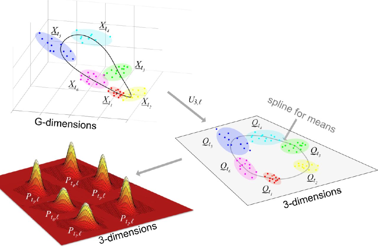
 are projected into d=3 dimensions using Ud,i to get
  . A MVN distribution is estimated for each
  and then these distributions are interpolated using splines to all times t of the day. See Fig. S4 for the projections Ud,i for the Bjarnason et al. data.
We fit a shape-preserving smoothing cubic periodic spline through the mean vectors μi(ti) and each of the six entries that determine the 3 × 3 symmetric matrix Σi(ti) so as to extend μi(ti) and Σi(ti) to all times t between the time points ti thus obtaining μi(ti) and Σi(ti). A piecewise cubic Hermite interpolating polynomial spline is used in this case. This type of spline is shape preserving, i.e. continuity of the second derivative is not obligatory. This is suitable as, for example, if two covariance matrix entries were identical for two consecutive time Gaussians, the Hermite spline allows the value of the joining spline to stay the same in the space between, while a standard spline would enforce some change. This spline also interpolates so that it passes through all points. The calculations were carried out using the MATLAB function pchip. Using this approach, for this value of i, we have determined a family of MVN distributions for all times t between the first and last data times.
Now we define the likelihood curve LX(t) where X is a G-dimensional normalised expression vector using the same genes as the TimeTeller panel. This is given by firstly defining the likelihood LX,i(t) associated with the ith timepoint using the probability given by the MVN i.e.
 and then combining them as follows

In Fig. S3 we explain why we use this local approach, using projections calculated locally and then combining them, rather than using a single projection of all the training data.
Construction of the clock dysfunction metric Θ
We characterise precision using ideas from statistics and information theory. If T is the time at which LX(t) is maximal (Fig. 1C,D), and we wish to consider the hypothesis that the time t of the sample is different from T then the Neyman-Pearson lemma tells us how to proceed. According to it, for a given significance level (i.e. probability of a false positive), the most powerful test uses the size of the likelihood ratio Λ(t) = LX(t)/LX(T) and is a test of the form Λ(t)≥η where η is chosen so as to obtain a given false-positive error rate. We choose a value of η and then define the clock dysfunction metric Θ to be the relative fraction of the times t for which Λ(t)≥η once we have chosen η. If Θ is small then LX(t) determines the time T with high certainty and we interpret this as the clock working well, but if it is large then LX(t) does not determine the time well and we interpret this as showing a dysfunctional clock.
However, the following considerations lead us to use a slightly more complicated approach. We explain in Fig. S4 that the likelihood LX(t) often has two peaks with another high peak roughly 12 hours away from the MLE. This is because of the elliptic form of our probability distribution in G-dimensional space (Fig. S4). In this case we would want the metric to penalise the lesser peak, but if the two peaks are close then we would not want this penalty because that is compatible with reasonably good clock function (see Fig. S6). As it stands, the metric would not distinguish between these two cases.
In view of this, rather than using a constant threshold η we use one that is a function of time t, namely, we multiply η by C(t | T,ϵ) where C(t | T,ϵ) = 1 + ϵ + cos(2π (t − T) / 24). This is a simple cosine curve transformed so that ϵ ≤ C ≤ 2 + ϵ, C(T | T,ϵ) = ϵ and C(T + 12 | T,ϵ)) = 2 + ϵ. We define ϵ > 0 so that C > 0. The larger ϵ is, the less anti-phase peaks impact the final confidence metric. The values of η and used are explained in the Note S4.
The clock dysfunction metric Θ is defined to be the proportion of times t which satisfy

Some examples of likelihoods and how we would want them to be classified are shown in Fig. S6.
Finally, we note that the above definition does not use the value of the likelihood at its maximum. To ensure that the maximum value achieved is not too small and that exceptionally small values are discounted, we set a minimum value ω for the likelihoods and we reset LX(t) to LX(t) = ω whenever LX(t)≤ ω. The parameter ω reflects the perceived signal-to-noise ratio. It means that the value of the likelihood curve at the MLE must be far greater than this limit for it to be significant, i.e. LX(T) ≫ ω. A typical value used for ω is e−5 ≈ 0.0067 and this value was chosen manually, by observation of the log-likelihood curves.
Author Contribution Statement
FL and DAR conceived the project and supervised it. DV developed the algorithm and analysed the data under the guidance of DAR. DV wrote the initial draft under the supervision of DAR and FL. DAR carried out further analysis and wrote the manuscript with assistance from DV, FL & SG. SG provided all data connected with the REMAGUS 2 trial and provided advice on breast cancer. GB provided the dataset used for parameterising the human version of TimeTeller. All authors contributed to and approved the manuscript.
Acknowledgements
We thank Ida Iurisci (INSERM U776, Villejuif) for help with complementary information regarding the breast cancer database and Meritxell Saez (University of Warwick) for a critical reading. DAR and DV thank the Engineering & Physical Sciences Research Council (EPSRC) for a PhD studentship through the MOAC Doctoral Training Centre grant number EP/F500378/1. DAR was also supported by Biotechnology and Biological Sciences Research Council (BBSRC) Grant BB/K003097/1 and EPSRC Grant EP/P019811/1. FL & DAR were supported by a grant from Cancer Research UK and EPSRC (C53561/A19933). GAB was supported by The Anna-Liisa Farquharson Chair in Renal Cell Cancer Research.


