

Abstract
A central goal in systems neuroscience is to understand the functions performed by neural circuits. Previous top-down models addressed this question by comparing the behaviour of an ideal model circuit, optimised to perform a given function, with neural recordings. However, this requires guessing in advance what function is being performed, which may not be possible for many neural systems. Here, we propose an alternative approach that uses recorded neural responses to directly infer the function performed by a neural network. We assume that the goal of the network can be expressed via a reward function, which describes how desirable each state of the network is for carrying out a given objective. This allows us to frame the problem of optimising each neuron’s responses by viewing neurons as agents in a reinforcement learning (RL) paradigm; likewise the problem of inferring the reward function from the observed dynamics can be treated using inverse RL. Our framework encompasses previous influential theories of neural coding, such as efficient coding and attractor network models, as special cases, given specific choices of reward function. Finally, we can use the reward function inferred from recorded neural responses to make testable predictions about how the network dynamics will adapt depending on contextual changes, such as cell death and/or varying input statistics, so as to carry out the same underlying function with different constraints.
INTRODUCTION
Neural circuits have evolved to perform a range of different functions, from sensory coding to muscle control and decision making. A central goal of systems neuro-science is to elucidate what these functions are and how neural circuits implement them. A common ‘top-down’ approach starts by formulating a hypothesis about the function performed by a given neural system (e.g. efficient coding/decision making), which can be formalised via an objective function [1–10]. This hypothesis is then tested by comparing the predicted behaviour of a model circuit that maximises the assumed objective function (possibly given constraints, such as noise/metabolic costs etc.) with recorded responses.
One of the earliest applications of this approach was sensory coding, where neural circuits are thought to efficiently encode sensory stimuli, with limited information loss [7–13]. Over the years, top-down models have also been proposed for many central functions performed by neural circuits, such as generating the complex patterns of activity necessary for initiating motor commands [3], detecting predictive features in the environment [4], or memory storage [5]. Nevertheless, it has remained difficult to make quantitative contact between top-down model predictions and data, in particular, to rigorously test which (if any) of the proposed functions is actually being carried out by a real neural circuit.
The first problem is that a pure top-down approach requires us to hypothesise the function performed by a given neural circuit, which is often not possible. Second, even if our hypothesis is correct, there may be multiple ways for a neural circuit to perform the same function, so that the predictions of the top-down model may not match the data.
Here, we propose an approach to directly infer the function performed by a recurrent neural network from recorded responses. To do this, we first construct a top-down model describing how a recurrent neural network could optimally perform a range of possible functions, given constraints on how much information each neuron encodes about its inputs. A reward function quantifies how useful each state of the network is for performing a given function. The network’s dynamics are then optimised to maximise how frequently the network visits states associated with a high reward. This framework is very general: different choices of reward function result in the network performing diverse functions, from efficient coding to decision making and optimal control.
Next, we tackle the inverse problem of infering the reward function from the observed network dynamics. To do this, we show that there is a direct correspondence between optimising a neural network as described above, and optimising an agent’s actions (in this case, each neuron’s responses) via reinforcement learning (RL) [14–18] (Fig 1). As a result, we can use inverse RL [19–23] to infer the objective performed by a network from recorded neural responses. Specifically, we are able to derive a closed-form expression for the reward function optimised by a network, given its observed dynamics.

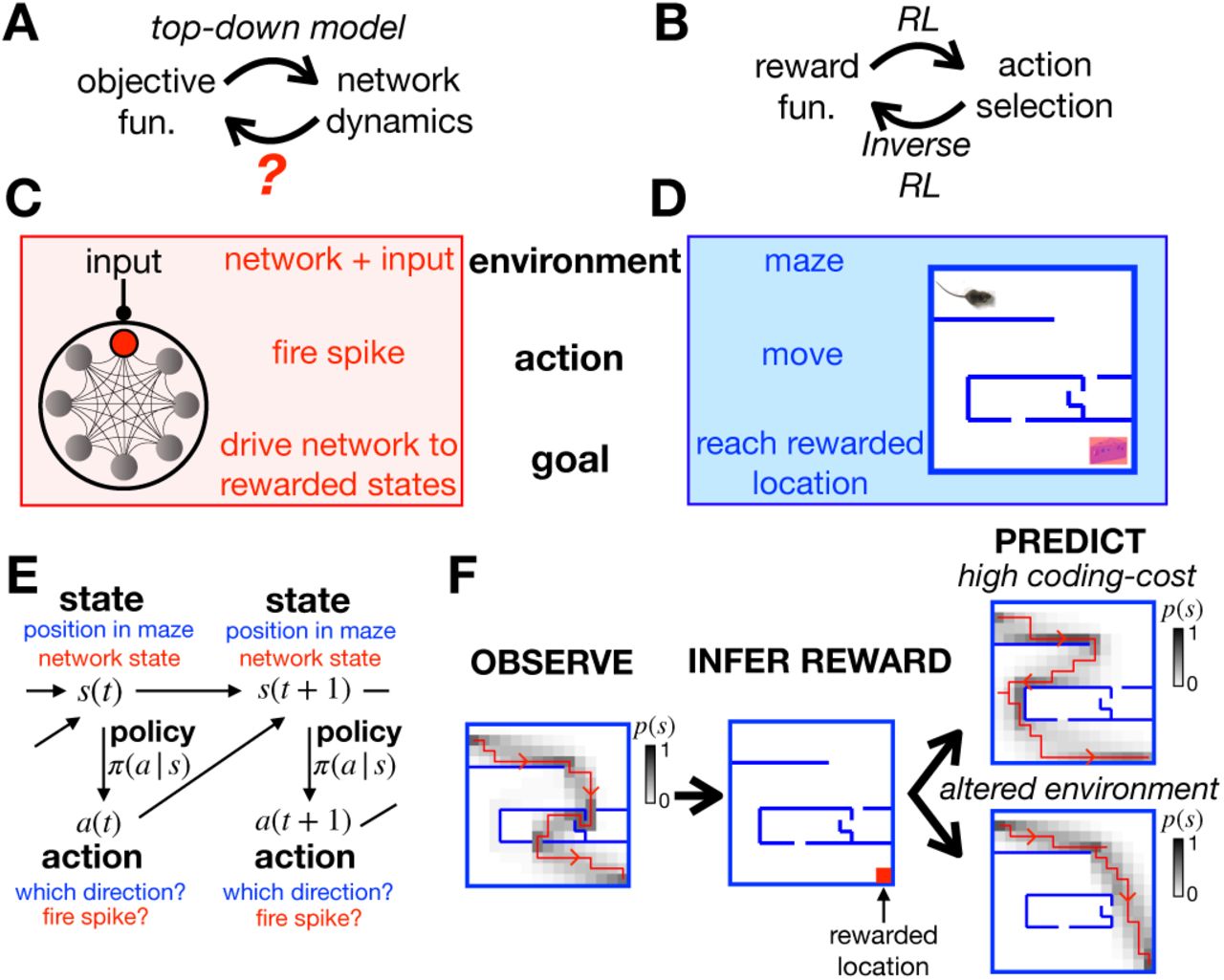
(A) Top-down models use an assumed objective function to derive the optimal neural dynamics. Here we address the inverse problem, to infer the objective function from observed neural responses. (B) Similarly, RL uses an assumed reward function to derive an optimal set of actions that an agent should perform in a given environment, while inverse RL infers the reward function from the agent’s actions. (C-D) A mapping between the neural network and textbook RL setup. (E) Both problems can be formulated as MDPs, where the agent (or neuron) can choose which actions, a, to perform to alter their state, s, and increase their reward. (F) Given a reward function and coding cost (which penalises complex policies), we can use entropy-regularised RL to derive the optimal policy (left). Here we plot a single trajectory sampled from the optimal policy (red), as well as how often the agent visits each location (shaded). Conversely, we can use inverse RL to infer the reward function from the agent’s policy (centre). We can then use the inferred reward to predict how the agent’s policy will change when we increase the coding cost to favour simpler (but less rewarded) trajectories (top right), or move the walls of the maze (bottom right).
We hypothesise that the inferred reward function, rather than e.g. the properties of individual neurons, is the most succinct mathematical summary of the network, that generalises across different contexts and conditions. Thus we can use our framework to quantitatively predict how the network will adapt or learn in order to perform the same function when the external context (e.g. stimulus statistics), constraints (e.g. noise level) or the structure of the network (e.g. due to cell death or experimental manipulation) change. Our framework thus not only allows RL to be used to train neural networks and use inverse RL to infer their function, but it also generates predictions for a wide range of experimental manipulations.
RESULTS
General approach
We can quantify how well a network performs a specific function (e.g. sensory coding/decision making) via an objective function Lπ (where π denotes the parameters that determine the network dynamics) (Fig 1A). There is a large literature describing how to optimise the dynamics of a neural network, π, so as to maximise a specific objective functions, Lπ, given constraints (e.g. metabolic cost/wiring constraints etc.) [1–10]. However, it is generally much harder to go in the opposite direction, to infer the objective function, Lπ, from observations of the neural network dynamics.
To address this question, we looked to the field of reinforcement learning (RL) [14–18], which describes how an agent should choose actions so as to maximise the reward they receive from their environment (Fig 1B). Conversely, another paradigm, called inverse RL [19–23], explains how to go in the opposite direction, to infer the reward associated with different states of the environment from observations of the agent’s actions. We reasoned that, if we could establish a mapping between optimising neural network dynamics (Fig 1A) and optimising an agent’s actions via RL (Fig 1B), then we could use inverse RL to infer the objective function optimised by a neural network from its observed dynamics.
To illustrate this idea, let us compare the problem faced by a single neuron embedded within a recurrent neural network (Fig 1C) to the textbook RL problem of an agent navigating a maze (Fig 1D). The neuron’s environment is determined by the activity of other neurons in the network and its external input; the agent’s environment is determined by the walls of the maze. At each time, the neuron can choose whether to fire a spike, so as to drive the network towards states that are ‘desirable’ for performing a given function; at each time, the agent in the maze can choose which direction to move in, so as to reach ‘desirable’ locations, associated with a high reward.
Both problems can be formulated mathematically as Markov Decision Processes (MDPs) (Fig 1E). Each state of the system, s (i.e. the agent’s position in the maze, or the state of the network and external input), is associated with a reward, r(s). At each time, the agent can choose to perform an action, a (i.e. moving in a particular direction, or firing a spike), so as to reach a new state s′ with probability, p(s′|a, s). The probability that the agent performs a given action in each state, π(a |s), is called their policy.
We assume that the agent (or neuron) optimises their policy to maximise their average reward, , given a constraint on the information they can encode about their state, Iπ(a; s) (this corresponds, for example, to constraining how much a neuron can encode about the rest of the network and external input). This can be achieved by maximising the following objective function:
 where λ is a constant that controls the strength of the constraint. Note that in the special case where the agent’s state does not depend on previous actions (i.e. p (s′|a, s) = p (s′|s)) and the reward depends on their current state and action, this is the same as the objective function used in rate-distortion theory [24, 25]. We can also write the objective function as:
 where cπ(s) is a ‘coding cost’, equal to the Kullback-Leibler divergence between the agent’s policy and the steady-state distribution over actions, DKL [π (a |s) ‖pπ (a)]. In SI section 1A we show how this objective function can be maximised via entropy-regularised RL [15, 18] to obtain the optimal policy:
 where ν π (s) is a ‘value function’ defined as the predicted reward in the future (minus the coding cost) if the agent starts in each state (SI section 1A):
 where s, s′ and s″ denote three consecutive states of the agent. Thus, actions that drive the agent towards high reward (and thus, high value) states are preferred over actions that drive the agent towards low reward (and thus, low value) states.
Let us return to our toy example of the agent in a maze. Figure 1F (left) shows the agent’s trajectory through the maze after optimising their policy to maximise Lπ. In this example, a single location, in the lower-right corner of the maze, has a non-zero reward (Fig 1F, centre). However, suppose we didn’t know this; could we infer the reward at each location just by observing the agent’s trajectory in the maze? In SI section 1A we show that this can be done by finding the reward function that maximises the log-likelihood of the optimal policy, averaged over observed actions and states, ⟨log π * (a |s) ⟩data. If the coding cost is non-zero (λ > 0), this problem is well-posed, meaning there is a unique solution for r(s).
Once we know the reward function optimised by the agent, we can then use it to predict how their behaviour will change when we alter their external environment or internal constraints. For example, we can predict how the agent’s trajectory through the maze will change when we move the position of the walls (Fig 1F, lower right), or increase the coding cost so as to favour simpler (but less rewarded) trajectories (Fig 1F, upper right).
Optimising neural network dynamics
We used these principles to infer the function performed by a recurrent neural network. We considered a model network of n neurons, each described by a binary variable, σi = −1/1, denoting whether the neuron is silent or spiking respectively (SI section 1B). The net-work receives an external input, x. The network state is described by an n-dimensional vector of binary values, σ = (σ1, σ2, …, σn)T. Both the network and external input have Markov dynamics. Neurons are updated asynchronously: at each time-step a neuron is selected at random, and its state updated by sampling from  . The dynamics of the network are fully specified by the set of transition probabilities,
  , and input statistics, p(x′| x).
As before, we use a reward function, r (σ, x), to express how desirable each state of the network is to perform a given functional objective. For example, if the objective of the network is to faithfully encode the external input, then an appropriate reward function might be the negative squared error:  , where
  denotes an estimate of x, inferred from the network state, σ. More generally, different choices of reward function can be used to describe a large range of functions that may be performed by the network.
The dynamics of the network, π, are said to be optimal if they maximise the average reward,  , given a constraint on the information each neuron encodes about the rest of the network and external inputs,
  . This corresponds to maximising the objective function:
 where λ controls the strength of the constraint.
For each neuron, we can frame this optimisation problem as an MDP, where the state, action, and policy correspond to the network state and external input {σ, x}, the neuron’s proposed update  , and the transition probability
  , respectively. Thus, we can use entropy-regularised RL to optimise each neuron’s response probability,
  , exactly as we did for the agent in the maze. Further, as each update increases the objective function Lπ, we can alternate updates for different neurons to optimise the dynamics of the entire network. In SI section 1B, we show that this results in transition probabilities given by:
 where σ/i is the state of all neurons except neuron i, and
 where vπ (σ, x) is the value associated with each state, defined in Eqn 4, with a coding cost,
  , which penalises deviations from each neuron’s average firing rate. The network dynamics are optimised by alternately updating the value function and neural response probabilities (SI section 1B).
To see how this works in practice, we simulated a network of 8 neurons that receive a binary input x (Fig 2A). The assumed goal of the network is to fire exactly 2 spikes when x = −1, and 6 spikes when x = 1, while minimising the coding cost. To achieve this, the reward was set to unity when the network fired the desired number of spikes, and zero otherwise (Fig 2B). Using entropy-regularised RL, we derived optimal tuning curves for each neuron, which show how their spiking probability should vary depending on the input, x, and number of spikes fired by other neurons (Fig 2C). We confirmed that after optimisation the number of spikes fired by the network was tightly peaked around the target values (Fig 2D). Decreasing the coding cost reduced noise in the network, decreasing variability in the total spike count.
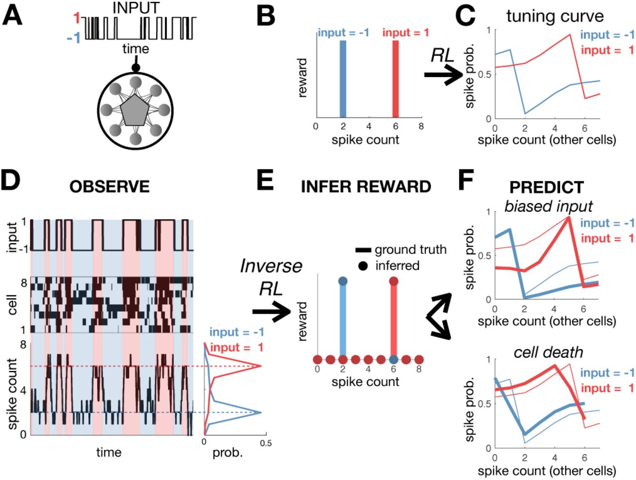
(A) A recurrent neural network receives a binary input, x. (B) The reward function equals 1 if the network fires 2 spikes when x = −1, or 6 spikes when x = 1. (C) The optimal neural tuning curves depend on the input, x, and total spike count. (D) Simulated dynamics of the network with 8 neurons (left). The total spike count (below) is tightly peaked around the rewarded values. (E) Using inverse RL on the observed network dynamics, we infer the original reward function used to optimise the network from its observed dynamics. (F) The inferred reward function is used to predict how neural tuning curves will adapt depending on contextual changes, such as varying the input statistics (e.g. decreasing p(x = 1)) (top right), or cell death (bottom right). Thick/thin lines show adapted/original tuning curves, respectively.
Inferring the objective function from the neural dynamics
We next asked if we could use inverse RL to infer the reward function optimised by a neural network, just from its observed dynamics (Fig 2D). For simplicity, we first consider a recurrent network that receives no external input, in which case the optimal dynamics (Eqn 6) correspond to Gibbs sampling from a steady-state distribution:  . Combining this with the Bellmann equality (which relates the value function, vπ (σ, x), to the reward function, r (σ, x)), we can derive the following expression for the reward function:
 where p (σi|σ/i) denotes the probability that neuron i is in state σi, given the current state of all the other neurons and C is an irrelevant constant. Note that using the wrong coding cost, λ, will rescale the reward by the same factor, and thus rescale the objective function without changing its shape. SI section 1C shows how we can recover the reward function when there is an external input. In this case, we do not obtain a closed-form expression for the reward function, but must instead infer it via maximum likelihood.
Figure 2E shows how we can use inverse RL to infer the reward function optimised by a model network from its observed dynamics. As for the agent in the maze, once we know the reward function, we can use it to predict how the network dynamics will vary depending on the internal/external constraints. For example, we can predict how neural tuning curves vary when we alter the input statistics (Fig 2F, upper), or kill a cell (Fig 2F, lower).
Application to a pair-wise coupled network
Our framework is limited by the fact that the number of states, ns, scales exponentially with the number of neurons (ns = 2n). Thus, it quickly becomes infeasible to compute the optimal dynamics as the number of neurons increases. Likewise, we need an exponential amount of data to reliably estimate the sufficient statistics of the network, required to infer the reward function.
This problem can be circumvented by using a tractable parametric approximation of the value function. For example, if we approximate the value function by a quadratic function of the responses our framework predicts a steady-state response distribution of the form:  , where Jij denotes the pair-wise coupling between neurons, and hi is the bias. This corresponds to a pair-wise Ising model, which has been used previously to model recorded neural responses [26, 27]. In SI section 1D we derive an approximate RL algorithm to optimise the coupling matrix, J, for a given reward function r (σ) and coding cost.
To illustrate this, we simulated a network of 12 neurons arranged in a ring, with reward function equal to 1 if exactly 4 adjacent neurons are active together, and 0 otherwise. After optimisation, nearby neurons had positive couplings, while distant neurons had negative couplings (Fig 3A). The network dynamics generated a single hill of activity which drifted smoothly in time. This is reminiscent of ring attractor models, which have been influential in modeling neural functions such as the rodent and fly head direction system [28–30].
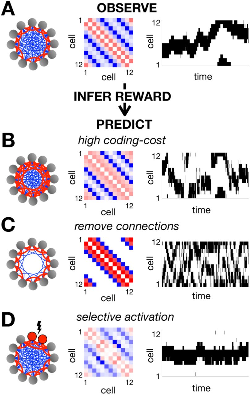
(A) We optimized the parameters of a pair-wise coupled network, using a reward function that was equal to 1 when exactly 4 adjacent neurons were simultaneously active, and 0 otherwise. The resulting couplings between neurons are schematized on the left, with positive couplings in red and negative couplings in blue. The exact coupling strengths are plotted in the centre. On the right we show an example of the network dynamics. Using inverse RL, we can infer the original reward function used to optimise the network from its observed dynamics. We can then use this inferred reward to predict how the network dynamics will vary when we increase the coding cost (B), remove connections between distant neurons (C) or selectively activate certain neurons (D).
As before, we could then use inverse RL to infer the reward function from the observed network dynamics. However, note that when we use a parametric approximation of the value function this problem is not well-posed, and we have to make additional assumptions (SI section 1D). In our simulation, we found that assuming that the reward function was both sparse and positive was sufficient to recover the original reward function used to optimise the network (SI section 2C).
Having inferred the reward function optimised by the network, we can use it to predict how the coupling matrix, J, and network dynamics vary depending on the internal/external constraints. For example, increasing the coding cost resulted in stronger positive couplings between nearby neurons and a hill of activity that sometimes jumped discontinuously between locations (Fig 3B); removing connections between distant neurons resulted in two uncoordinated peaks of activity (Fig 3C); finally, selectively activating certain neurons ‘pinned’ the hill of activity to a single location (Fig 3D).
Inferring efficiently encoded stimulus features
An influential hypothesis, called ‘efficient coding’, posits that sensory neural circuits have evolved to encode maximal information about sensory stimuli, given internal constraints [7–13]. However, the theory does not specify which stimulus features are relevant to the organism, and thus should be encoded. Here we show how one can use inverse RL to: (i) infer which stimulus features are encoded by a recorded neural network, and (ii) test whether these features are encoded efficiently.
Efficient coding posits that neurons maximise information encoded about some relevant feature, y (x), given constraints on the information encoded by each neuron about their inputs, x (Fig 4A). This corresponds to maximising:
 where λ controls the strength of the constraint. Noting that the second term is equal to the coding cost we used previously (Eqn 5), we can rewrite this objective function as:
 where we have omitted terms which don’t depend on π. Now this is exactly the same as the objective function we have been using so far (Eqn 5), in the special case where the reward function, r (σ, x), is equal to the log-posterior, log pπ (y (x) |σ). As a result we can maximise Lπ via an iterative algorithm, where on each iteration we update the reward function by setting r (x, σ) ← log pπ(y (x) |σ), before then optimising the network dynamics, via entropy-regularised RL. Thus, thanks to the correspondence between entropy-regularised RL and efficient coding we could derive an algorithm to optimise the dynamics of a recurrent network to perform efficient coding [27].

(A) The neural code was optimised to efficiently encode an external input, x, so as to maximise information about a relevant stimulus feature y (x). (B) The input, x consisted of 7 binary pixels. The relevant feature, y (x), was equal to 1 if >4 pixels were active, and −1 otherwise. (C) Optimising a network of 7 neurons to efficiently encode y (x) resulted in all neurons having identical tuning curves, which depended on the number of active pixels and total spike count. (D) The posterior probability that y = 1 varied monotonically with the spike count. (E) The optimised network encoded significantly more information about y (x) than a network of independent neurons with matching stimulus-dependent spiking probabilities, p (σi = 1|x). The coding cost used for the simulations in the other panels is indicated by a red circle. (F-G) We use the observed responses of the network (F) to infer the reward function optimised by the network, r (σ, x) (G). If the network efficiently encodes a relevant feature, y (x), then the inferred reward (solid lines) should be proportional to the log-posterior, log p (y (x) |σ) (empty circles). This allows us to (i) recover y (x) from observed neural responses, (ii) test whether this feature is encoded efficiently by the network. (H) We can use the inferred objective to predict how varying the input statistics, by reducing the probability that pixels are active, causes the population to split into two cell types, with different tuning curves and mean firing rates (right).
As an illustration, we simulated a network of 7 neurons that receive a sensory input consisting of 7 binary pixels (Fig 4B, top). Here, the ‘relevant feature’, y (x) was a single binary variable, which was equal to 1 if more than 4 pixels were active, and −1 otherwise (Fig 4A, bottom). Using the efficient-coding algorithm described above, we derived optimal tuning curves, showing how each neuron’s spiking probability should vary with both the number of active pixels and number of spikes fired by other neurons (Fig 4C). We also derived how the optimal readout, p (y |σ), depended on the number of spiking neurons (Fig 4D). Finally, we checked that the optimised network encoded significantly more information about the relevant feature than a network of independent neurons, over a large range of coding costs (Fig 4E).
Now, imagine that we just observe the stimulus and neural responses (Fig 4F). Can we recover the relevant feature, y (x)? To do this, we first use inverse RL to infer the reward function from observed neural responses (Fig 4G). As described above, if the network is performing efficient coding then the inferred reward, r (σ, x) should be proportional to the log-posterior, log p (y (x)|σ). Thus, given σ, the inferred reward, r (σ, x) should only depend on changes to the input, x, that alter y (x). As a result, we can use the inferred reward to uncover all inputs, x, that map onto the same value of y (x). Here, we see that the inferred reward collapses onto two curves only (blue and red in Fig 4G), depending on the total number of pixels in the stimulus. This allows us to deduce that the relevant coded variable, y (x), must be a sharp threshold on the number of simultaneously active pixels (despite the neural tuning curves varying smoothly with the number of active pixels; Fig 4C). Next, having recovered y (x), we can check whether it is encoded efficiently by seeing whether the inferred reward, r (σ, x) is proportional to the logposterior, log p (y (x) |σ).
Finally, once we have inferred the function performed by the network, we can predict how its dynamics will vary with context, such as when we alter the input statistics. For example, in our simulation, reducing the probability that input pixels are active causes the neural population to split into two cell-types, with distinct tuning curves and mean firing rates (Fig 4H) [13].
DISCUSSION
A large research effort has been devoted to developing ‘top-down’ models, which describe the network dynamics required to optimally perform a given function (e.g. decision making [6], control [3], efficient sensory coding [8] etc.). Here, we go in the opposite direction: starting from recorded responses, we show how to infer the objective function optimised by the network. This approach, where the objective function is inferred from data, should allow one to: (i) quantitatively predict the responses of a given recorded network, from functional principles; (ii) build top-down models of high-level neural areas, whose function is a priori unknown.
An alternative bottom-up approach is to construct phenomenological models describing how neurons respond to given sensory stimuli and/or neural inputs [26, 27, 31, 32]. In common with our work, such models are directly fitted to neural data. However, unlike our work, they do not set out to reveal the function performed by the network. Further, they are often poor at predicting neural responses in different contexts (e.g. varying stimulus statistics). Here we hypothesize that it is the function performed by a neural circuit that remains invariant, not its dynamics or individual cell properties. Thus, if we can infer what this function is, we should be able to predict how the network dynamics will adapt depending on the context, so as to perform the same function under different constraints. As a result, our theory could predict how the dynamics of a recorded network will adapt in response to a large range of experimental manipulations, such as varying the stimulus statistics, blocking connections, knocking out/stimulating cells etc.
There is an extensive literature on how neural networks could perform RL [33–35]. Our focus here was different: we sought to use tools from RL and inverse RL to infer the function performed by a recurrent neural network. Thus, we do not assume the network receives an explicit reward signal: the reward function is simply a way of expressing which states of the network are useful for performing a given function. In contrast to previous work, we treat each neuron as an independent agent, which optimises their responses to maximise the reward achieved by the network, given a constraint on how much they can encode about their inputs. As well as being required for biological realism, the coding constraint has the benefit of making the inverse RL problem well-posed. Indeed, under certain assumptions, we show that it is possible to write a closed form expression for the reward function optimised by the network, given its steady-state distribution (Eqn 8).
Our framework relies on several assumptions about the network dynamics. First, we assume that the network has Markov dynamics, such that its state depends only on the preceding time-step. To relax this assumption, we could redefine the network state to include spiking activity in several time-steps. For example, we could thus include the fact that neurons are unlikely to fire two spikes within a given temporal window, called their refractory period. Of course, this increase in complexity would come at the expense of decreased computational tractability, which may necessitate approximations. Second, we assume the only constraint that neurons face is a ‘coding cost’, which limits how much information they encode about other neurons and external inputs. In reality, biological networks face many other constraints, such as the metabolic cost of spiking and constraints on the wiring between cells, which we may want to incorporate explicitly into our framework in the future.
Our work unifies several influential theories of neural coding, that were considered separately in previous work. For example, we show a direct link between entropy-regularised RL [15–18] (Fig 1), ring-attractor networks [28–30] (Fig 3), and efficient sensory coding [7–13] (Fig 4). Further, given a static network without dynamics, our framework is directly equivalent to ratedistortion theory [24, 25]. While interesting in its own right, this generality means that we can potentially apply our theory to infer the function performed by diverse neural circuits, that have evolved to perform a broad range of different functional objectives. This contrasts with previous work, where neural data is typically used to test a single top-down hypothesis, formulated in advance.
ACKNOWLEDGMENTS
This work was supported by ANR JCJC grant (ANR-17-CE37-0013) to M.C, ANR Trajectory (ANR-15-CE37-0011), ANR DECORE (ANR-18-CE37-0011), the French State program Investissements d’Avenir managed by the Agence Nationale de la Recherche (LIFESENSES; ANR-10-LABX-65), EC Grant No. H2020-785907 from the Human Brain Project (SGA2), and an AVIESAN-UNADEV grant to O.M. The authors would like to thank Ulisse Ferrari for useful discussions and feedback.


