

Abstract
We analysed the genomic architecture of neuroanatomical diversity using magnetic resonance imaging and SNP data from > 20,000 individuals. Our results replicate previous findings of a strong polygenic architecture of neuroanatomical diversity. SNPs captured from 40% to 54% of the variance in the volume of different brain regions. We observed a large correlation between chromosome length and the amount of phenotypic variance captured, r∼0.64 on average, suggesting that at a global scale causal variants are homogeneously distributed across the genome. At a more local scale, SNPs within genes (∼51%) captured ∼1.5-times more genetic variance than the rest; and SNPs with low minor allele frequency (MAF) captured significantly less variance than those with higher MAF: the 40% of SNPs with MAF<5% captured less than one fourth of the genetic variance. We also observed extensive pleiotropy across regions, with an average genetic correlation of rG∼0.45. Across regions, genetic correlations were in general similar to phenotypic correlations. By contrast, genetic correlations were larger than phenotypic correlations for the left/right volumes of the same region, and indistinguishable from 1. Additionally, the differences in left/right volumes were not heritable, underlining the role of environmental causes in the variability of brain asymmetry. Our analysis code is available at https://github.com/neuroanatomy/genomic-architecture.
Introduction
Twin and extended pedigree studies have have shown the variability of various neuroanatomical structures to be heritable up to h2∼80% (Blokland et al. 2012; Wen et al. 2016). These estimations have been followed up by a series of studies on unrelated subjects which, based on whole-genome genotyping data, have estimated an heritability of up to h2∼55% (Toro et al. 2015; Hibar et al. 2015). Genome-wide association studies (GWAS) aiming at identifying associated variants through international collaborative efforts such as ENIGMA and CHARGE have revealed, however, only few statistically significant associated loci (Stein et al. 2012; Hibar et al. 2015; Satizabal et al. 2017). These results are compatible with the hypothesis of a highly polygenic architecture, where phenotypes are influenced by large numbers of loci of effect sizes too small to reach genome-wide significance (usually p<5×10⁻⁸). This hypothesis has been supported by the findings of several research groups (Toro et al. 2015; Ge et al. 2015, 2016; Zhao et al. 2018; Elliott et al. 2018), thanks to the development of methods to estimate heritability and genetic correlation from whole-genome genotyping data (reviewed by Yang et al. 2017).
In a previous work (Toro et al. 2015) we used a sample of N=2,011 subjects with whole-genome genotyping data from the IMAGEN consortium combined with structural magnetic resonance imaging (MRI) data analysed according to the pipelines of the ENIGMA consortium, and showed that genome-wide SNPs were able to capture a substantial proportion of the variability in regional brain volume – up to 55% ± 25%. The advent of the UK Biobank project, in particular, has allowed researchers to greatly increase the number of subjects used for heritability estimation (see for example, Elliott et al 2018, Zhao et al 2018). Here we replicate and follow up on these results using a sample ten times larger, N=26,818, including data from the UK Biobank project as well as 5 other projects that had previously participated in the ENIGMA consortium (IMAGEN, SHIP, TREND, Lothian, ADNI).
We measured the same regional brain volumes as in the ENIGMA consortium studies by Stein et al (2012) and Hibar et al (2015): several subcortical structures, total brain volume and intracranial volume. In addition, we also studied height and intelligence scores. Brain volume correlates with height and intelligence scores (Taki et al. 2012), which are both known to be heritable (Yang et al. 2010; Plomin and Deary 2015). We aimed thus at determining to which extent the heritability of regional brain volumes was given by its relationship with height (i.e., affected by the same genetic factors that determine body size), or if different genetic factors affected them specifically. Similarly for intelligence scores, we aimed at better understanding its relationship with brain volume.
For all phenotypes, we estimated how much genome-wide SNPs were able to capture the inter-individual variability in regional brain volumes, that is, we estimated the proportion of phenotypic variance captured by SNPs across the whole genome (also called SNP heritability). Additionally, we used our GWAS data to compute genome-wide polygenic scores, which provide a phenotypic prediction at the individual level. The analyses of the influence of the complete genome on our phenotypes were complemented with analyses on a series of genomic partitions: genic versus non-genic; preferential expression in the central nervous system; low, medium or high minor allele frequency. This can reveal whether specific genomic regions have a particularly large effect on phenotypic variability. Finally, we looked at the pleiotropy across phenotypes. We computed genetic correlations and phenotypic correlations for all pair of phenotypes, and for brain regions, we compared in particular to the genetic and phenotypic correlations between the left and side parts of the same structure as a mean to estimate the role of genetics and environment in brain asymmetry. All our estimations were computed for each project independently, and combined together meta-analytically.
Methods
Data sharing
We obtained whole-genome genotyping from N=26,818 subjects from 6 different projects: UK Biobank, IMAGEN, ADNI, Lothian Birth Cohort 1936, SHIP and TREND. The UK Biobank project (https://imaging.ukbiobank.ac.uk) is a large, long-term biobank study in the United Kingdom aiming at investigating the contributions of genetic predisposition and environmental exposure to the development of disease. The study is following about 500,000 volunteers enrolled at ages from 40 to 69 years old, 54% females. IMAGEN (https://imagen-europe.com) is a project to identify and characterise specific genetically-influenced alterations in reinforcer sensitivity and executive control which are manifest in adolescence and carry the risk for overt psychopathology later in life. It includes general population 13 to 17 years old adolescents (49% of females) from Germany, France, Ireland, and the United Kingdom. ADNI, the Alzheimer’s Disease Neuroimaging Initiative (http://adni.loni.usc.edu), is a longitudinal multicenter study designed to develop clinical, imaging, genetic, and biochemical biomarkers for the early detection and tracking of Alzheimer’s disease in the United States of America. The dataset combines data from the initial five-year study (ADNI-1), and the follow-ups ADNI-GO, ADNI-2, and ADNI-3. It includes subjects 54 to 90 years old, 42% female. The Lothian Birth Cohort 1936 (https://www.lothianbirthcohort.ed.ac.uk) is a follow-up of the Scottish Mental Surveys of 1947, which tested the intelligence of almost every child born in 1936 and attending school in Scotland in the month of June 1947. It includes subject 71 to 73 years old, 47% female. The SHIP and TREND cohorts contain data from the Study of Health in Pomerania (SHIP, http://www2.medizin.uni-greifswald.de/cm/fv/ship.html), a population-based epidemiological study consisting of two independent cohorts SHIP and SHIP-TREND. These projects investigate common risk factors, subclinical disorders and diseases in a population of northeast Germany. The dataset included data from subjects 21 to 90 years old, 44% female for TREND, 48% female for SHIP. All data sharing was approved by our local ethical board as well as by those of the participating projects wherever required. The list of projects and their respective number of subjects is described in Table 1.
Sample sizes and number of variants per project. *The UK Biobank dataset was split in two parts: N=14,144 subjects were used for heritability analyses (13,086 included), and N=6,678 subjects were used for validation of genome-wide polygenic scores (6,184 included).
Regional brain volumes
The measurements of regional brain volume coming from projects that had previously participated in ENIGMA (IMAGEN, Lothian Birth Cohort 1936, TREND, SHIP and ADNI) were the same that had been used in Stein et al (2012) and Hibar et al (2015). For the UK Biobank subjects, the estimation of the volumes were performed using FreeSurfer 6.0 (https://surfer.nmr.mgh.harvard.edu). We also included for comparison the estimations using FSL FIRST (https://fsl.fmrib.ox.ac.uk/fsl) that were made available by UK Biobank (the processing pipeline is described in https://biobank.ctsu.ox.ac.uk/crystal/docs/brain_mri.pdf). In addition to the subjects excluded in the quality control made by the UK Biobank, we excluded 52 additional subjects showing an extreme relationship between total brain volume and intracranial volume. For this, we used a kernel density estimator to fit a probability density function to the intracranial versus brain volume data, and tagged as outliers all subjects in with a local density inferior to 1% of the maximum density for UK Biobank, and 2% for other datasets.
The regions included in our analyses were: nucleus accumbens (labelled as Acc), amygdala (Amy), putamen (Pu), pallidum (Pa), caudate nucleus (Ca), hippocampus (Hip) and thalamus (Th); along with brain volume (BV) and intracranial volume (ICV). In addition to these regions, we investigated height and intelligence scores (IS), available from the UK Biobank and IMAGEN projects. It is important to note that the fluid intelligence score in UK Biobank (a 2 minutes test aiming at evaluating the capacity to solve problems that require logic and reasoning ability, independent of acquired knowledge; see https://biobank.ctsu.ox.ac.uk/crystal/label.cgi?id=100027), is not the same as the intelligence score used by the IMAGEN project, which was obtained using the WISC test.
Genotype filtering
All genetic analyses were performed for each project independently. The genotyping data was converted to the hg19 reference wherever required using UCSC LiftOver (http://genome.ucsc.edu/cgi-bin/hgLiftOver). We used genotyped autosomal SNPs (single nucleotide polymorphisms) which passed UK Biobank quality control for all batches (http://www.ukbiobank.ac.uk/wp-content/uploads/2014/04/UKBiobank_genotyping_QC_documentation-web.pdf). Additionally, we removed SNPs in 24 regions with long range linkage disequilibrium (LD, see Price et al. 2008). SNPs were then filtered to exclude those with minor allele frequency (MAF) <0.1%, missing rate >1%, or Hardy-Weinberg disequilibrium with a p<10−6. Individuals were removed when >10% of their SNPs were missing. We finally pruned SNPs which were in linkage disequilibrium with a variance inflation factor >10, which corresponds to a multiple R2 for the regression over linked SNPs <0.9. The filtering was made using PLINK v1.90b3.46 (Purcell et al. 2007).
Genetic relationship matrices (GRM)
GRMs were computed based on autosomal chromosomes using GCTA v1.91.3 (Yang, Lee, et al. 2011). We included only one of each pair of subjects with an estimated relatedness >0.025 (approximately corresponding to cousins two to three times removed). GRMs were computed per chromosome and then merged for the whole genome.
Population structure
Genetic variance estimations based on genomic estimates of relatedness are sensitive to cryptic relatedness and population structure. These factors can influence the phenotypic similarity beyond the estimated degree of genetic relatedness (Yang, Manolio, et al. 2011; Browning and Browning 2011). In addition to the exclusion of subjects with a degree of genetic relatedness greater than 0.025 (that is, more related than third or fourth cousins), we used the first 10 principal components of the GRM as covariates in our statistical analyses.
Genetic variance
We estimated the amount of phenotypic variance captured by SNPs using a linear mixed model with age, sex, imaging centre, and the first 10 principal components of the GRM as fixed effect covariates, and a random effect with a covariance matrix corresponding to the GRM (GCTA GREML method, Yang et al. 2011). We estimated SNP heritability as the ratio of the genetic variance to the phenotypic variance, with genetic variance being the variance of the random component, and the phenotypic variance being the sum of random component and residual component with fixed effects removed. We used GCTA v1.91.3 (Yang, Lee, et al. 2011) for those computations and did not constrain genetic variance estimations in order to obtain unbiased estimates (option --reml-no-constrain).
Genetic correlation
Genetic correlation was estimated using GCTA REML bivariate analysis (Lee, Yang, et al. 2012) in constrained mode (option --reml-bivar). Both phenotypic and genetic correlation were adjusted for age, sex, imaging centre, and the first 10 principal components of the GRM unless specified in the manuscript. We compared genetic and phenotypic correlations using the delta method to estimate standard errors (R package msm). We report estimations with their standard errors (s.e.).
Genetic variance partitioning
In its simplest form, GCTA allows to estimate the amount of variance captured by the matrix of genetic relationships, assuming that each SNP captures the same amount of variance. Through genomic partitions we can create different genetic relationship matrices based on non-overlapping regions of the genome. The SNPs on each of these partitions can capture then a different amount of variance (although, as before, SNPs within a same partition are supposed to capture all the same amount of variance).
We grouped SNPs based on the partitions used in Toro et al (2015)
Partition based on genic status. Using 66,632 gene boundaries from the UCSC Genome Browser hg19 assembly, we made a first set with all SNPs within these boundaries, two further sets that included also SNPs 0 to 20 kbp and 20kbp to 50 kbp upstream and downstream of each gene, and a last set including the SNPs not located in regions less than 50 kbp upstream or downstream of genes. These partitions do not correspond exactly to those used by Toro et al (2015). The previous partitions were one with strict genic/non-genic boundaries (0 kbp), another with genic ± 20 kbp versus the rest, and finally genic ± 50 kbp versus the rest.
Partition based on preferential central nervous system (CNS) expression (Raychaudhuri et al.2010; Lee, DeCandia, et al. 2012) using ± 50 kbp as gene boundaries.
Partition based on allele frequency. A partition based on MAF with 4 groups: from 0.1 to 5%, from 5 to 20%, from 20 to 35% and from 35 to 50%. In the original article, only the last 3 partitions were included, covering the range from 5 to 50% of MAF.
Partition genetic variance enrichment
Once the variance captured by each partition is computed, we can estimate the significance of the difference in variance captured by an individual partition against a model where each SNP captures exactly the same amount of variance. In this latter case, the amount of variance capture by each partition should be directly proportional to the number of SNPs it contains.
We first aimed to assess the statistical significance of the partition enrichment using a permutation test as in Toro et al (2015) and a derivation of statistical significance obtained from the covariance matrix of variance estimates reported by GCTA.
In the permutation test, SNPs were randomly selected to build the partitions, keeping the same number of SNPs as in the original partition. For each set of random partitions, the same linear mixed-effects model as before was fitted (including age, sex, centre and 10 PCs). We tested whether any of these partitions captured more variance than what could be expected given its number of SNPs. Briefly, a Z-score was computed by comparing the SNP-set genetic estimated variance  of partition i to the SNP-set genetic variance
  expected under no enrichment:
 where f i is the fraction of the SNPs included in partition i. The p-value of enrichment was computed by comparing the observed Z score to those obtained from 1,000 permutations.
One limitation of this approach is that it does not preserve the local LD relationships among SNPs. We observed that the standard errors of the genetic variance estimates reported by the permutation approach were systematically larger than those computed from the covariance matrix of variance estimates. To better preserve the original LD, we tried an alternative permutation method in which we permuted blocks of contiguous SNPs. For the partitioning based on genic status, the standard errors of the simulated partitions estimates were compatible with the standard error of the original partitions (Fig. S1). However, this alternative permutation method did not reduce the gap with the theoretical values for the partitioning by MAF since they depend only on the frequency of the individual SNPs, and not on their contiguity over the genome (Fig. S2). Because of this, and because the permutation approach was much more demanding in terms of computation, we decided to use only the theoretical derivation of enrichment test: We evaluated whether  was statistically significantly positive with a one-sided Z-test, considering that in the null hypothesis of no enrichment, each genomic partition should carry an amount of variance proportional to its number of SNPs. We estimated the variance of the observed enrichment using equation 2:

Here, represents the genetic variance of partition i and
  .
.
Meta-analysis
The independent estimations obtained from each of the projects were combined into a single one using an inverse variance weighting method. We validated the meta-analytical approach by comparing the distribution of genetic variance estimates from simulated heritable phenotypes with their theoretical normal distribution in sub-samples of ADNI and UK Biobank datasets.
Genome-wide polygenic scores
We used the SNP effects estimated in the association analysis from the 13,086 subjects of UK Biobank to estimate the phenotypes of 6,184 additional unrelated subjects with MRI data from the latest release of the UK Biobank. The scores were estimated from the filtered SNPs (not LD pruned). SNPs under various association p-value thresholds were selected and the ones in LD with a more significantly associated SNP were clumped. The p-value threshold that produced the best fit with the target dataset was selected. We used the software PRSice associated with plink for the computation of genome-wide polygenic scores (Euesden, Lewis, and O’Reilly 2015). We covaried out the effects of age, sex, imaging centre, and the 10 first principal components of the GRM. The analyses were performed on the residuals of this linear regression. We then estimated the variance captured by genome-wide polygenic scores using the coefficient of determination r2. For comparison, we also computed the predicted height of the 6,000 subjects using summary statistics of the GIANT GWAS (Wood et al. 2014; https://www.nature.com/articles/ng.3097), N=253,288. We used this to evaluate how more precise SNP effect estimates from a larger dataset could improve prediction.
Results
Genetic variance estimates
We obtained estimates of the ratio of total genetic variance to phenotypic variance (VG/Vp) for all projects. We did not constrain the estimates to lie between 0 and 100%. Estimates outside this range were often obtained when sample sizes were small. For example, for the Lothian project 4 out of the 9 brain region’s estimates were outside the 0% to 100% range, with 95% confidence intervals often encompassing the complete 0% to 100% range (Table S1.1, Fig. 1). The standard errors of the estimates greatly decreased with sample size, from about 76% for ∼550 individuals, 43% for ∼1,000 individuals, 24% for ∼1,750 individuals (IMAGEN), down to 4% for UK Biobank with more than 13,000 individuals. Our result from simulated phenotypes showed that the estimations of VG/VP on simulated phenotypes obtained with sub-samples of N=800, N=400, N=200 and even N=100 subjects from the UK Biobank project were unbiased relative to the expected normal distribution. The simulations based on the ADNI project, however, showed a significant bias towards positive values when the sub-samples included N=100 to N=400 subjects, probably due to the heterogeneity of the population (Figures S10-11 and Table S6-7).

Proportion of variance capture by common genotyped variants (VG/VP) for brain regions, height and intelligence score. Meta-analytic estimates were obtained using inverse variance weighting of the estimates of the different projects studied. b. VG/VP estimates for each project. The estimates were obtained using GCTA, without constraining the results to lie in the 0% to 100% range. The diamond shows the meta-analytic estimation. Age, sex, center, and the first 10 principal components were included as covariates. The error bars show the standard errors of the VG/VP estimates. Acc: nucleus accumbens, Amy: amygdala, Pu: putamen, Pa: pallidum, Ca: caudate nucleus, Th: thalamus, Hip: hippocampus, BV: brain volume, ICV: intracranial volume, IS: intelligence score (fluid intelligence for UK Biobank, full intelligence quotient for IMAGEN).
In all cases, the meta-analytic estimations (inverse variance weighted) closely corresponded with the values obtained for the UK Biobank project (Table S1.2), which because of its large sample size accounted for ∼94% of the weighted estimates. Standard errors agreed well with the theoretical values proposed by Visscher et al (2014), and implemented in the GREML statistical power calculator (http://cnsgenomics.com/shiny/gctaPower): they were from 1.01 to 1.05 times higher than the theoretical values when taking into account the variance of the genetic relationships, except for ADNI where they were 1.21 times higher).
Meta-analytic estimates of genetic variance are shown in Figure 1, which combine the results from all the independent projects we analysed. Estimates for intracranial volume and total brain volume were large: VG/VP(ICV) = 53 ± 4.5% (all our variance estimates are reported as estimation ± s.e.), VG/VP (BV) = 52 ± 4.5%). Similarly, the genetic variance estimates for subcortical structures were all above 40%: Accumbens (VG/VP = 40 ± 4.5%), amygdala (VG/VP = 45 ± 4.5%), putamen (VG/VP = 48 ± 4.5%), palladium (VG/VP = 40 ± 4.5%), caudate (VG/VP = 52 ± 4.5%), thalamus (VG/VP = 54 ± 4.5%), hippocampus (VG/VP = 53 ± 4.5%). All estimates were highly statistically significant with p<10−11 in all cases (log-likelihood ratio statistics from 49 to 242 in UK Biobank alone) (Fig. 1, Table S1.2). The VG/VP estimate for caudate nucleus (VG/VP = 52 ± 4.4%) was statistically significant and very different from what was observed in the IMAGEN cohort (VG/VP = 4 ± 24%) which, as mentioned in Toro et al (2015), may reflect an age bias specific to IMAGEN (individuals were on average 14 years old).
The meta-analytic VG/VP estimate for height (which combines only UKB and IMAGEN) was large: VG/VP = 71 ± 3.1% and close to those obtained from twin studies (Polderman et al. 2015) and from previous SNP heritability estimates (VG/VP = 68.5 ± 0.4% in (Ge et al. 2017)). The fluid intelligence score in UKB had the lowest heritability among all 11 studied phenotypes, VG/VP = 35 ± 4.8%. This estimate is similar to the one obtained by Davies et al. (2011) on 30,801 UKB subjects (VG/VP = 31% ± 1.8%). The verbal and performance intelligence scores (VIQ and PIQ) in IMAGEN, although not based on the same test as fluid intelligence (FI) in UK Biobank, aim at capturing a similar phenotype. The estimate for fluid intelligence in UK Biobank seem smaller than those for verbal and performance intelligence quotients in IMAGEN (∼56 ± 26%), however, they were not statistically significantly different.
Similarly to what we had observed previously (Toro et al. 2015), the genetic variance estimates were not significantly affected by population structure: the non-inclusion of the 10 first PCs did not impact the estimates of variance, which changed on average by less than 4% (Fig. S3).
Comparison of genetic variance estimates of the UK Biobank project across previous studies
Several recent studies have used the UK Biobank data to estimate genetic variance of regional brain volumes. The reported estimates vary across studies, with subcortical volumes, in particular the volume of the amygdala, showing the largest differences.
We compared our genetic variance estimates with those obtained by two recent studies (Elliott et al. 2018; Zhao et al. 2018). Zhao et al. (2018) used GCTA to compute VG/VP estimates of the left and right volumes of various subcortical structures on a smaller sample of 9,031 subjects from the UK Biobank project. Regional brain volumes were quantified using ANTs (Advanced Normalization Tools software (Avants et al. 2014) together with the MindBoggle-101 atlas (Klein and Tourville 2012). Elliott et al. (2018) reported genetic variance estimates for thousands of phenotypes on 8,411 subjects, using SBAT (Sparse Bayesian Association Test (Elliott et al. 2018)). These phenotypes included the volumes of subcortical structures that we report here. Elliott et al (2018) provide VG/VP estimates obtained from measurements of subcortical structures performed using FSL’s FIRST (FMRIB’s Integrated Registration and Segmentation Tool (Patenaude et al. 2011)) and FreeSurfer. In the original study of the IMAGEN data we reported only total volumes (left plus right) computed using FIRST. For the sake of comparison, we computed VG/VP estimates in the UK Biobank data for the left and right volumes separately, using both FIRST and FreeSurfer (Table S2).
The largest difference of hemispheric variance estimates was observed for the amygdala and the nucleus accumbens (Fig. 2), which are the smallest structures of those we studied. These structures also displayed the lowest correlation between right and left volumes (Fig. S4) and between FIRST and FreeSurfer measurements (Fig. S5), which suggests that their measurement may be less precise than for larger structures. A similar discrepancy between left and right amygdala volume was observed by both Zhao et al. (2018) and Elliott et al. (2018) (Fig. 2). Discrepancies between VG/VP estimates were more important when comparing different methods to estimate subcortical volumes (FreeSurfer, FIRST, or MindBoggle/ANTs) than when comparing different methods to estimate genetic variance (GCTA or SBAT). The inclusion of the brain volume as a covariate did not change noticeably our variance estimates and thus could not fully explain the differences observed with the study of Zhao et al (2018) (Fig. S6). In all cases, however, 95% CIs built from the standard errors of each study contained the estimates of the other studies.

Comparison of our estimations of genetic variance (VG/VP) in the UK Biobank project with 2 recent studies: Elliot et al (2018) and Zhao et al (2018). VG/VP estimates were computed for brain, intracranial volume (ICV), and subcortical volumes of the right and left hemispheres measured using different methods (FreeSurfer, or MindBoggle/ANTs, FIRST) represented by the shapes of the dots. In yellow are represented the estimates of VG/VP we computed using GCTA REML unconstrained method, the other VG/VP estimates were published by Elliott et al. 2018 (green) and Zhao et al. 2018 (orange). Age, sex, center, and the top 10 principal components were included as covariates. The error bars show the standard errors of the VG/VP estimates.
We also compared our VG/VP estimates for the ADNI project with those obtained by Zhao et al. (2018). After filtering and merging of the non-imputed genotypes across the two ADNI sub-projects, we included 982 subjects and 210,543 SNPs; Zhao et al (2018) included 1,023 subjects and 7,368,446 SNPs (after imputation). Despite both analyses using the same covariates, the VG/VP estimates showed differences ranging from 7% to 99%. These differences are not surprising, however, given the small sample size, and thus the large standard errors of the estimates (Fig. S6).
Enrichment of genetic variance partitions
We partitioned the total genetic variance in different ways and computed the enrichment in variance captured by each partition relative to their number of SNPs. The following partitions were investigated:
Partition per chromosome (autosomes)
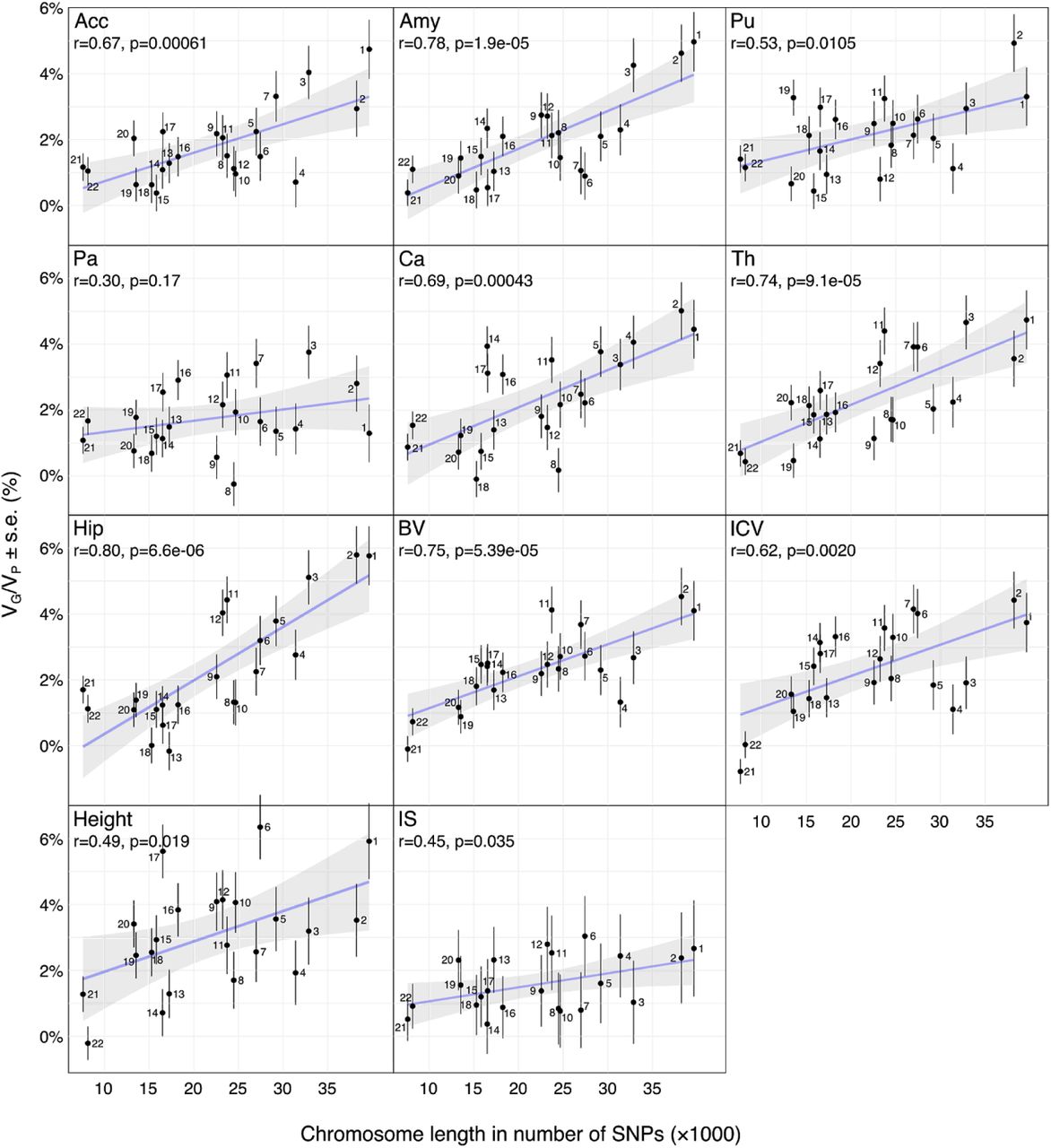
The correlation between VG/VP estimates and chromosome size was significant for all phenotypes except the pallidum (Fig. 3). The correlation coefficients ranged from 0.30 ± 0.21 to 0.80 ± 0.13, capturing on average 41% of the variance (estimated as r2).

Scatter plots of the number of SNPs per chromosome versus the VG/VP estimates computed for each chromosome independently. VG/VP estimates were obtained by partitioning SNPs across chromosomes and computed using the GCTA REML unconstrained method for total subcortical volumes. Age, sex, center, and the top 10 principal components were included as covariates. The error bars show the standard errors of the VG/VP estimates.
Partition between genic and non-genic regions
We first partitioned the total genetic variance into four sets of SNPs: those within gene boundaries, those located 0 to 20 kbp, those 20 kbp to 50 kbp upstream and downstream of each gene, and the rest. Across projects, the genic SNP set (± 0 kbp) contained 51% of all genotyped SNPs and captured on average 69% of the variance attributable to SNPs of most of the studied phenotypes, significantly more than what we would expect from its length (FDR < 5%). The only exceptions were fluid intelligence and nucleus accumbens, for which it explained respectively 59 ± 9% and 55 ± 6% of the total genetic variance (Fig. 4, Table S4). Height was the only phenotype for which we observed an enrichment of VG/VP captured by one of the non-genic SNP sets: the set of SNPs within 0 ± 20 kbp of the genic set. This set contained 15% of all SNPs but explained 27% of the variance of the height phenotype attributable to SNPs (FDR corrected p < 0.01). In total, the variants located between 0 and 50 kbp away from genes captured 36 ± 4% of the genetic variance of height (FDR corrected p < 0.05).

Variance enrichment for partitions based on closeness to genic regions. Top: VG/VP estimates computed for four sets of SNPs based on their distance to gene boundaries: all SNPs within the boundaries of the 66,632 gene boundaries from the UCSC Genome Browser hg19 assembly, two further sets that included also SNPs 0 to 20 kbp and 20kbp to 50 kbp upstream and downstream of each gene, and a remaining set containing SNPs located farther than 50kb from one of the gene boundaries. VG/VP estimates were computed using the GCTA REML unconstrained method for height, intelligence, and brain, intracranial and total subcortical volumes. The error bars represent the standard errors. Bottom: Enrichment of variance captured by each partition. The y-axis shows the ratio of the fraction of genetic variance explained by each partition divided by the fraction of SNPs contained in each partition. If all SNPs explained a similar amount of variance, this ratio should be close to 1 (dashed line). A Z-test was used to compare the ratios to 1 and p-values were FDR adjusted (*p<0.05, **p<0.01, ***p<0.001).
Partition by involvement in preferential CNS expression
No statistical enrichment was found when comparing the genetic variance between SNP sets overlapping and not overlapping with functional annotations (genes involved in central nervous system function (Raychaudhuri et al. 2010; Lee, DeCandia, et al. 2012)). All results of VG/VP partitioning are available in Table S3 and Table S4.
Partition by allele frequency
We grouped SNPs in four different partitions based on their MAF: (1) 0.1% to 5% (40% of SNPs), (2) 5% to 20% (30% of SNPs), (3) 20% to 35% (12% of SNPs), and (4) 35% to 50% (9% of SNPs). We observed that SNPs within the low MAF partition (MAF<5%) captured less genetic variance than those with medium and high MAF (the 3 partitions with MAF>5%) (Fig. 5), as previously described by Speed et al (2017). The partition of SNPs with low MAF contained 40% of the SNPs, however, it captured on average only about 16% of the total genetic variance. This is less than expected in the GCTA model where each SNP captures the same amount of phenotypic variance, but slightly more than expected in a neutral theory of evolution, where the captured variance is proportional to the size of the MAF bin (Yang et al. 2017; Visscher et al. 2012).

Variance enrichment for partitions based on minor allele frequency (MAF). Top: VG/VP estimates computed for four sets of SNPs based on their MAF: from 0.1 to 5%, from 5 to 20%, from 20 to 35% and from 35 to 50%. VG/VP estimates were computed using the GCTA REML unconstrained method for height, intelligence, and brain, intracranial and total subcortical volumes. The error bars represent the standard errors. Bottom: Enrichment of variance captured by each partition. The y-axis shows the ratio of the fraction of genetic variance explained by each partition divided by the fraction of SNPs contained in each partition. If all SNPs explained a similar amount of variance, this ratio should be close to 1 (dashed line). A Z-test was used to compare the ratios to 1 and p-values were FDR adjusted (*p<0.05, **p<0.01, ***p<0.001).
Genetic and phenotypic correlations among traits
We computed phenotypic and genetic correlation matrices for the UK Biobank project, shown in figure Fig. 6 (Table S5). Genetic correlations represent the correlation between genetic effects of two phenotypes.

UK Biobank data. Values of phenotypic (A) and genetic (B) correlations are shown in the lower triangles. Circles in the upper triangles have a diameter proportional to the strength of the correlation, and a thickness proportional to the size of the confidence interval. Stars indicate statistical significance of the correlation being non null (*P<0.05, **P<0.01, ***P<0.001). C. Scatter plot of phenotypic versus genetic correlations. The following phenotypes are represented: the volumes of accumbens (Acc), amygdala (Amy), brain, caudate (Cau), hippocampus (Hip), pallidum (Pa), putamen (Pu), and thalamus (Th); height and intelligence score (IS) are also represented. Phenotypic correlations were adjusted for age, center, and sex. Genetic correlations were adjusted for age, center, sex, and the top 10 principal components of the genetic relationship matrix.
We had previously observed (Toro et al. 2015) that the correlation between brain volume and intelligence scores was higher than the correlation between brain volume and height. Here, the genetic correlation between height and brain volume was significant, rG = 0.164 ± 0.053, and smaller than the genetic correlation between brain volume and intelligence: rG = 0.343 ± 0.080. However, the difference was not statistically significant: rG:BV.FI -rG:BV.height = 0.179 ± 0.095, 95% CI:, −0.008, 0.365 (computed using the formula xxxvii in Pearson and Filon (1898)). The correlations between fluid intelligence and height – phenotypic and genetic – were the smallest we observed across all phenotypes: rP = 0.101 ± 0.009 and rG = 0.048 ± 0.073.
In general, the concordance between phenotypic and genetic correlation was high (R2 = 0.80, Fig 6.C), as reported by Sodini et al (2018) for other traits, and the correlation matrices were similar (Figure S7). When considering total volumes, differences between genetic and phenotypic correlations were not different from zero (Z-test FDR > 50%, Table S5). When considering the left and right hemispheres separately, however, the genetic correlations between the left and right parts of each subcortical structure were not statistically different from rG = 1 and were different from the phenotypic correlations (Z-test FDR < 5%, Figure S9 and Table S5), reflecting the influence of environment in hemispheric asymmetry. To test this hypothesis, we measured the VG/VP of the differences between left and right volumes of each structure. Only the heritability of the difference in volume of the left and right accumbens was significantly different from zero (VG/VP = 16 ± 4.5). Except for this structure, the differences in volumes between right and left hemispheres of all the other brain regions seemed to be only environmental.
Prediction using genome-wide polygenic scores
Finally, we computed the genome-wide polygenic scores for ∼6,000 additional participants from the UK Biobank who were not used for the heritability estimate. Genome-wide polygenic scores captured a very small, although statistically significant proportion of the phenotypic variance, ranging from 0.5% (p < 10e-22) for the amygdala to 2.2% (p<10e-31) for brain volume (Figure S13, Figure S14, and Supplemental Table S8). For height, a genome-wide polygenic score obtained based on GWAS summary statistics from ∼13k UK Biobank subjects captured ∼3% of the variance. To evaluate the impact of the number of samples used in the GWAS on the amount of variance captured by the genome-wide polygenic score, we also computed the genome-wide polygenic scores using the GWAS summary statistics from the GIANT consortium (N∼250k). This allowed to capture ∼17% of the variance of height (almost 6-times more) (Figure S15).
Discussion
Our results confirmed that a substantial proportion of the diversity in regional brain volume is captured by genome-wide SNPs, that the genetic architecture of this effect seems to be highly polygenic, and that SNPs close to genic regions capture a significantly higher proportion of the variability than the rest of the genome. The estimates we obtained were similar to our original results (Toro et al. 2015). Thanks to data sharing, and the recent availability of the UK Biobank project data, we were able to collect a sample size more than 10-times larger than the one used in the original study, which greatly increased the precision of our estimates. All our scripts have been released open source to facilitate further replication and extension of our results.
Whole-genome frequent variants captured a substantial proportion of the variability in regional brain volumes, ranging from 40% (pallidum) to 55% (thalamus). The genomic architecture of neuroanatomical diversity appeared to be strongly polygenic: a partition of variance per chromosome showed a significant correlation between chromosomal size and the amount of variance captured. The regression between chromosomal length and heritability captured on average 63% of the variance in their relationship. Only a very small fraction of this variance could be captured by genome-wide polygenic scores.
We confirmed the genetic correlation between total brain volume, intelligence scores, and height, however, we did not find evidence for a significantly higher genetic correlation between brain volume and intelligence scores compared with the genetic correlation between brain volume and height.
Additionally, we observed that SNPs with higher minor allele frequency captured in average more variance that those with lower minor allele frequency, and that genetic correlations between the left and right parts of a same region were significantly higher than the phenotypic correlations, suggesting an important effect of environmental, non-genetic factors in shaping brain asymmetry.
Genic regions and those immediately adjacent presented a statistically significant enrichment in variance captured for all phenotypes, with the exception of intelligence. Overall, a genic variant would capture about two times more variance than a non-genic variant. The partitions of SNPs with medium to high minor allele frequency (MAF>5%) captured proportionally more variance than the one with low MAF. Despite low per-SNP heritability, the per-SNP effect sizes have been shown to be on average higher for SNPs with low MAF, in accordance with a model of negative selection (the relationship between captured heritability h2 and allele effect b for a given SNP is h2 = 2· b2 · f · (1 -f), with f being the allele frequency. See Schoech et al. 2017; and Zeng et al. 2018).
The genetic correlation between height and brain volume was not significantly different from the genetic correlation between intelligence scores and brain volume, contrary to what we had observed previously (Toro et al. 2015). The genetic correlation between height and intelligence scores was, however, the smallest across all phenotypes, suggesting that their relationship with brain volume may be due to different genetic factors.
The sources of brain asymmetry may be mostly due to non-genetic, environmental factors. The genetic correlations between the left and right parts of the same brain regions were in general indistinguishable from rG=1. Their phenotypic correlations, however, although strong, were statistically significantly smaller. Only for one brain region, the nucleus accumbens, did the asymmetry in volume seem to have a partly genetic source.
The difficulty to accurately segment small, poorly defined, subcortical structures such as the amygdala or the nucleus accumbens, may explain the large differences in volume measurements and hence the differences in heritability estimates that we reported when comparing segmentation methods. The method used to measure volumes had a larger impact on the estimations of genetic variance than the method used for the estimation of heritability. Large volume differences both between manual and automated segmentation and between FreeSurfer and FIRST segmentations have been previously reported, in particular for the amygdala (Morey et al. 2009; Schoemaker et al. 2016).
Rather than combining our genetic datasets into a single one, we chose to estimate the part of phenotypic variance captured by SNPs independently in each dataset and then combine estimates in a meta-analysis. While our chosen solution helps to handle heterogeneity, it trades on statistical power. The reason for this is that the standard error of the GCTA GREML heritability estimate is approximately inversely proportional to the number of subjects (Visscher et al. 2014) (Figure S13).
In the present analysis, the UK Biobank project accounted for ∼94% of the estimations, largely driving the results. Indeed, the standard error of the estimates based on the UK Biobank project were reduced only by a factor of ∼1.03 through the inclusion of the other projects. If the raw genotyping data had been combined in a single mega-analysis instead of in a meta-analysis, the decrease in standard error would have been ∼1.36 smaller than what we reported. The meta-analytical approach may prove interesting in the future, however, with availability of large imaging genetics datasets other than UK Biobank, as well as in cases where raw genotyping data cannot be easily shared.
Genome-wide polygenic scores computed from GWAS summary statistics on ∼13k subjects captured a very small, although statistically significant proportion of the variance. For brain volume, for example, they captured ∼2.5% of the variance, for a SNP heritability of more than 50%. This is the expected result in presence of a strongly polygenic phenotype (Wray et al. 2013). It is also expected that the prediction accuracy will improve as the number of subjects increases. In the case of height, by using 250k subjects instead of 13k, the amount of variance captured increased from ∼3% to ∼17%. The UK Biobank project will provide at term a sample of 100k subjects with MRI data, which should allow us similarly to increase the amount of regional volume variance that genome-wide polygenic scores can capture to ∼12% (based on Wray et al. 2013 and Daetwyler, Villanueva, and Woolliams 2008).
Our results support to the hypothesis of a strongly polygenic architecture of human neuroanatomical diversity. They confirming our original findings (Toro et al. 2015) as well as those of others (Elliott et al. 2018; Zhao et al. 2018), and provide new information on the genetic bases of brain asymmetry. The importance of strongly polygenic architectures in the determination of physiological and anthropometric phenotypes is now well documented (Ge et al. 2017), as is their influence on various cognitive phenotypes as well as the risk to develop several psychiatric conditions (Zhang et al. 2018). The detection of candidate genes of large effect is an appealing tool for gaining mechanistic insight on normal and pathological phenotypes. However, this approach is ill adapted to strongly polygenic architectures, where not only a few large-effect alleles are involved, but potentially hundreds of thousands of alleles of almost infinitesimal effect (Wray et al. 2018). Neuroimaging endophenotypes such as those obtained using structural and functional MRI can provide a powerful, relevant, alternative source of mechanistic insight. The brain imaging literature is rich in examples of associations between different brain regions and networks with normal and pathological cognitive phenotypes. The automatic mining of these associations could provide a layer of annotation for brain regions and networks similar to those available today for genome annotation. Further investigation of the genomic architecture of neuroimaging endophenotypes should prove an important tool to better understand the biological bases of brain diversity and evolution in humans, as well as the biological bases of the susceptibility to psychiatric disorders.
Acknowledgements
This work was supported by the Institut Pasteur; Center for Research and Interdisciplinarity (CRI), Centre National de la Recherche Scientifique (CNRS); the University Paris Diderot; the Fondation pour la Recherche Médicale [DBI20141231310]; the European Commission Horizon 2020 [COSYN]; The Human Brain Project; the European Commission Innovative Medicines Initiative [AIMS2-TRIALS; No. 777394]; the Cognacq-Jay foundation; the Bettencourt-Schueller foundation; the Orange foundation; the FondaMental foundation; the Conny-Maeva foundation; and the Agence Nationale de la Recherche (ANR) [SynPathy]; the Laboratory of Excellence GENMED (Medical Genomics) grant no.
ANR-10-LABX-0013, Bio-Psy; by the INCEPTION program ANR-16-CONV-0005, managed by the ANR part of the Investment for the Future program.
J.-B.P. was partially funded by NIH-NIBIB P41 EB019936 (ReproNim) NIH-NIMH R01 MH083320 (CANDIShare) and NIH 5U24 DA039832 (NIF), as well as the Canada First Research Excellence Fund, awarded to McGill University for the Healthy Brains for Healthy Lives initiative.
The Study of Health in Pomerania (SHIP) is part of the Community Medicine Research net (CMR) (http://www.medizin.uni-greifswald.de/icm) of the University Medicine Greifswald, which is supported by the German Federal State of Mecklenburg-West Pomerania. MRI scans in SHIP and SHIP-TREND have been supported by a joint grant from Siemens Healthineers, Erlangen, Germany and the Federal State of Mecklenburg-West Pomerania. This study was further supported by the EU-JPND Funding for BRIDGET (FKZ:01ED1615).
Footnotes
↵* Equal contribution
↵★ Equal contribution
↵† Data used in preparation of this article were obtained from the Alzheimer’s Disease Neuroimaging Initiative (ADNI) database (adni.loni.usc.edu). As such, the investigators within the ADNI contributed to the design and implementation of ADNI and/or provided data but did not participate in analysis or writing of this report. A complete listing of ADNI investigators can be found at: http://adni.loni.usc.edu/wp-content/uploads/how_to_apply/ADNI_Acknowledgement_List.pdf


