

Abstract
Intraspecific trait variation is caused by genetic and plastic responses to environment. This intraspecific diversity is captured in immense natural history collections, giving us a window into trait variation across continents and through centuries of environmental shifts. We measured phenotypes on a 216-year time series of Arabidopsis thaliana accessions from across the native range. We applied spatially varying coefficient models to quantify region-specific trends in trait coordination and trait responses to climate gradients. All traits exhibited significant change 15 across space and/or through time. For example, δ15N decreased over time across much of the range and leaf C:N increased, consistent with predictions based on anthropogenic changes in land use and atmosphere. Plants were collected later in the growing season in more recent years in many regions, possibly because populations shifted toward more spring germination and summer flowering as opposed to fall germination and spring flowering. When climate variables were considered, collection dates were earlier in warmer years, while summer rainfall had opposing associations with collection date depending on regions. There was modest correlation among traits, indicating that there is not a single life history/physiology axis. Nevertheless, leaf C:N was low for summer- versus spring-collected plants, consistent with a life history-physiology axis from slow-growing winter annuals to fast-growing spring/summer annuals. Regional heterogeneity in phenotype trends indicates complex responses to spatiotemporal environmental gradients potentially due to geographic genetic variation and climate interactions with other aspects of environment. Our study demonstrates how natural history collections can be used to broadly characterize trait responses to environment, revealing heterogeneity in response to anthropogenic change.
Introduction
An organism’s fitness is determined by the interaction between its traits and its environment. Organisms respond to environmental gradients in diverse ways, including genetic and plastic shifts in life history, phenology, and physiology (Burghardt, Metcalf, Wilczek, Schmitt, & Donohue, 2015; Reich, 2014; Wright et al., 2004). Spatial and temporal environmental gradients can promote phenotypic plasticity or generate varying selection across which populations adapt to local conditions (Bradshaw, 1965; Henn et al., 2018; Joshi et al., 2001; Leimu & Fischer, 2008; Linhart & Grant, 2002; Matesanz, Gianoli, & Valladares, 2010; Turesson, 1922). By studying how phenology and physiology change across environments through space and time we learn about mechanisms of adaptive environmental response and biological constraints.
Anthropogenic global change has led to dramatic phenotypic changes in many organisms. For example, many species are shifting their ranges poleward and temperate spring phenology is advancing (Parmesan & Yohe, 2003). However, anthropogenic global change is multi-faceted, involving climate, nitrogen deposition, atmospheric CO2, and land use. Our understanding of the specific environmental drivers of phenotypic change has been hampered by insufficient datasets. Furthermore, many populations and species do not exhibit the stereotypic phenological and range shifts (Both et al., 2004; CaraDonna, Iler, & Inouye, 2014; Park et al., 2018). These diverse responses can be caused by geographic variation in the rate of environmental change or by intraspecific genetic variation, clouding our understanding of anthropogenic impacts.
Published studies provide multiple (and sometimes conflicting) hypotheses for phenotype responses to specific environmental gradients. Using large, multispecies datasets, Reich and colleagues argued that multiple aspects of leaf trait variation are coordinated to generate a single life history and physiology axis from fast to slow that also corresponds to changes in dominant vegetation types across environments (known as the Leaf Economic Spectrum, LES) (Reich, 2014; Reich et al., 2003; Wright et al., 2004). Although empirical community-wide turnover in mean traits across environments often follows LES predictions, it is unclear whether within species trait variation responds similarly (Anderegg et al., 2018; Hu et al., 2015; J. P. Wright & Sutton-Grier, 2012). The LES predicts that lower nitrogen concentration leaves (high C:N, low proportion N) are found in drier and in hotter areas, in part because of investment in non-photosynthetic leaf features, especially veins (Blonder, Violle, Bentley, & Enquist, 2011; Sack et al., 2012) or mesophyll cell walls (Easlon et al., 2014). Leaf nitrogen physiology is an important aspect of environmental response, since leaf nitrogen is critical to photosynthetic capacity (Evans, 1989; Stocking & Ongun, 1962) and photorespiration (Rachmilevitch, Cousins, & Bloom, 2004). At the community level, leaf N (proportion of mass) generally increases with mean annual temperature, at least below the highest latitudes (Ordoñez et al., 2009; Reich & Oleksyn, 2004), and increases with greater precipitation (Reich et al., 2003). Fast-growing plants, including many accessions of our study species, Arabidopsis thaliana (hereafter, Arabidopsis), are expected to invest more in photosynthetic capacity (N) and less in structural elements (C). Arabidopsis exhibits genetic variation that weakly corresponds to LES predictions (Easlon et al., 2014; Sartori et al., 2018), though little is known about trait variation in natural plants.
Isotopic signatures in tissue provide additional clues to organismal responses to environmental conditions. Δ13C, which measures discrimination against 13C in photosynthesis, is an indicator of pCO2 within leaves (Ci) relative to atmospheric pCO2(Ca) (Farquhar, O’Leary, & Berry, 1982). Ci declines when stomata are closed, which may be a conservative life history response to soil drying, while Ca declines with elevation. Thus, we expect Δ13C to increase in moist growing environments and decrease with elevation (Diefendorf, Mueller, Wing, Koch, & Freeman, 2010; Farquhar et al., 1982; Zhu, Siegwolf, Durka, & Körner, 2010). δ15N (the ratio of 15N to 14N) can be affected by the same resource acquisition traits as leaf proportion nitrogen (Stock & Evans, 2006). However, leaf N and δ15N may also reflect N deposition and biogeochemical cycling (e.g. Pardo et al. 2007), thus their variation may directly reflect changing environments rather than strictly biological traits. Under controlled conditions, leaf isotope and nutrient composition tend to exhibit high intraspecific genetic and plastic variation (Chardon, Barthélémy, Daniel-Vedele, & Masclaux-Daubresse, 2010; Nienhuis, Sills, Martin, & King, 1994), which may reflect adaptive potential in natural environments.
In seasonal locations, phenology shapes and is shaped by the environment a plant encounters during vulnerable stages. As with many plants, Arabidopsis development can be highly sensitive to moisture, temperature, and photoperiod (Burghardt et al., 2015; Wilczek et al., 2009). For example, although warmth can increase growth rates, many Arabidopsis genotypes require winter cold cues (known as vernalization) to transition to spring flowering. Phenology of many annual plants largely collapses to a life history-physiology axis between slow growing, late flowering populations and fast growing, early flowering populations. Plants with rapid life histories may have physiological traits tied to fast growth and resource acquisition (e.g. high stomatal conductance, high leaf area relative mass (Specific Leaf Area, or SLA)) (Lovell et al., 2013; McKay, Richards, & Mitchell-Olds, 2003; Reich, 2014; Sartori et al., 2018). Rapid development and reproduction can allow plants to escape drought, a strategy employed by some genotypes of Arabidopsis (McKay et al., 2003). Other plants exhibit traits characteristic of drought avoidance, such as minimizing water loss (e.g. through stomatal closure) and maximizing water uptake (Kenney, Mckay, Richards, & Juenger, 2014; Ludlow, 1989). Fast life histories can allow spring or summer annual life cycles, where a plant germinates and flowers within a single season, while slow life histories and vernalization requirements result in a winter annual cycle, where a plant germinates in the fall and flowers the following spring.
Standardized metrics are needed to compare ecologically relevant phenological variation among sites of different climate timing and at different latitudes. Photothermal units (PTUs) integrate developmental time under favorable temperatures and light across a growing season and account for much of the environmental influence on flowering dates in Arabidopsis (Brachi et al., 2010; Wilczek et al., 2009). Measures of developmental time standardized to environmental conditions can better capture genetic variation in development compared to raw flowering dates in Arabidopsis, the latter of which are strongly driven by environment (Brachi et al., 2010). Thus, PTUs may help reveal phenological adaptation along spatial and temporal environmental gradients.
Museum collections offer broadly distributed sampling in space and time to test the relationships between phenotypes and environment in nature (Lang, Willems, Scheepens, Burbano, & Bossdorf, 2018; Willis et al., 2017). Variation in herbarium collection dates can be a reliable proxy for variation in phenology (Davis, Willis, Connolly, Kelly, & Ellison, 2015; MacGillivray, Hudson, & Lowe, 2010; Miller-Rushing, Primack, Primack, & Mukunda, 2006). Here, we leverage the immense fieldwork underlying natural history collections to investigate how intraspecific diversity is structured through time and along spatiotemporal climate gradients. Specifically, we use thousands of Arabidopsis specimens that span over 200 years of sampling across Arabidopsis’ range in Eurasia and Northern Africa. We quantify the spatial patterns of Arabidopsis’ phenotypic variation along environmental gradients, which allows us to put temporal trends in context. We hypothesized that for natural Arabidopsis populations, phenotype-environment correlations would follow fast-slow predictions of LES and phenology traits (Table 1). We combine these records with global gridded climate data to ask three questions about Arabidopsis in nature:
To what degree does intraspecific trait variation among wild individuals fall along a single coordinated life history-physiology axis?
Do life history and physiology vary across spatial environmental gradients in long-term average conditions, suggesting adaptive responses consistent with the LES?
Have life history and physiology changed over the last two centuries? In particular, have changes tracked climate fluctuations, suggesting adaptive responses consistent with the LES?
Year trends are predicted due to elevated CO2, nitrogen deposition, or elevated temperatures. Citations for hypotheses: (Amundson et al., 20031; BassiriRad et al., 20032; Burghardt et al., 20153; Craine et al., 20094; Diefendorf et al., 20105; Drake, Hanson, Lowrey, & Sharp, 20176; Gill et al., 20027; McLauchlan, Ferguson, Wilson, Ocheltree, & Craine, 20108; Menzel et al., 20069; Ordoñez et al., 200910; Peñuelas et al., 200411; Reich, Hungate, & Luo, 200612; Seibt, Rajabi, Griffiths, & Berry, 200813; Sparks & Carey, 200614; Stock & Evans, 200615; I. J. Wright et al., 200416)
Materials & Methods
Samples
Our set of samples (N= 3159) included Arabidopsis thaliana herbarium and germplasm accessions with known collection date between 1794 and 2010 from the native range of Arabidopsis in Europe, the Middle East, Central Asia, and North Africa (Hoffmann, 2002). For each herbarium specimen (N=2711) we visually verified species identification and reproductive status as simultaneously flowering and fruiting. Samples that were only fruited/senesced, only flowering, or had neither open flowers nor fruits were excluded to focus on a relatively uniform developmental stage (see Supplementary Table 1). This consistency is important for assessing C:N, since progression of plant development involves reallocation of nutrients, and for a meaningful characterization of phenology with collection date. Furthermore, too few samples (136/2711) were in other phenological stages to allow for a rigorous comparison. We excluded dozens of misidentified specimens, highlighting the importance of verification of information in natural history collections (cf. unverified data in some online databases). Wild-collected germplasm accessions with known collection date and location (N = 448) were included from the Arabidopsis Biological Resource Center (https://abrc.osu.edu/).
Leaf traits
To test LES hypotheses for response to environment, we measured Δ13C, δ15N, and C:N from leaf tissue of herbarium samples. We removed and pulverized leaf samples (mean weight = 2.75 mg) of a subset of our quality-checked herbarium specimens and sent them to the UC-Davis Stable Isotope Facility. In total, we obtained values for δ15N, δ13C, C:N, and proportion N in 456 accessions, although 3 samples were missing proportion N values. δ13C and 1 sample was missing both C:N and proportion N values.
We measured leaf δ13C (isotope ratio), but atmospheric δ13C has changed dramatically over the time period of this study due to fossil fuel emissions. Thus we converted leaf isotope ratio (δ13C) to discrimination (Δ13C) using an estimate of the atmospheric δ13C time series (McCarroll & Loader, 2004) from 1850 to 2000, continuing linear extrapolation beyond 2000, using the 1850 value for earlier specimens, and the equation of Farquhar et al. (1989),  , where δa is the isotope ratio in the atmosphere and δp is the isotope ratio in plant tissue (ratios relative to a standard).
Phenology
To estimate accumulated photothermal units (PTU) at date of collection, we used the equation of Burghardt et al. (2015) to model the hourly temperature values for the accumulation of sunlight degree hours between January 1 and dusk on the date of collection at each accession’s coordinate. Daylength was approximated with the R package geosphere (Hijmans, 2017). Monthly temperature values for the period 1900-2010 came from the Climate Research Unit time series dataset (New, Hulme, & Jones, 2000). PTUs were only calculated for specimens collected after 1900 due to the historical limit of the monthly temperature data. Daily temperatures were interpolated from monthly temperatures using the function splinefun in R on the “periodic” setting.
Statistical analysis
Arabidopsis displays substantial genetic diversity in environmental response between genotypes from different regions (e.g. Exposito-Alonso et al., 2018; Lasky, Forester, & Reimherr, 2018). Thus, we employed a regression model with spatially varying coefficients (generalized additive models, GAMs) to account for regional differences in responses to environment, much of which may have a genetic component (Wheeler & Waller, 2009; Wood, 2006). GAMs allow fitting of parameters that vary smoothly in space (i.e. parameter surfaces) and can thus capture spatially varying relationships between predictors and the response of interest. The spatially varying coefficients fit by GAM allow us to infer from the data where relationships between variables change, as opposed to binning data into a set of fixed (and possibly artificially defined) regions.
We selected climate variables based on knowledge of critical Arabidopsis developmental times and likely environmental stressors: average temperature in April, when warmth is expected to accelerate development (AprilMean in the models), minimum temperature in January, when vernalization cues are likely accumulating or when Mediterranean plants are in early growth (JanMinimum), and July aridity index (AI), when summer drought may be most likely (Fournier-Level et al., 2013; Hoffmann, 2002; Lasky et al., 2012; Wilczek, Cooper, Korves, & Schmitt, 2014). Our analyses are likely not highly sensitive to the exact calendar month chosen, given the high correlation in conditions between consecutive months (e.g. warm Aprils tend to be followed by warm Mays). Aridity index was calculated from July precipitation divided by July potential evapotranspiration (PET) (United Nations Environment Program, 1997). These climate gradients were generally not strongly correlated (July Aridity to April Mean Temperature r2 = 0.09; July Aridity to January Minimum Temperature r2 = 0.003; January Minimum Temperature to April Mean Temperature r2 = 0.4 by linear regression). We took temperature, precipitation, and PET values from the Climate Research Unit time series dataset, using values for the year of collection (New et al., 2000).
To assess how phenotypes have changed across the last few centuries (Question 3), we first tested a model with spatially-varying coefficients for the effect of year, allowing for geographic variation in temporal trends (hereafter, “year models”). The model also included spatially varying intercepts (SVI) to account for regional differences in long-term mean phenotypes. Year models included all specimens with phenotype data.
Next, to assess how temporal fluctuations in climate drive phenotypic change (Question 3), we fit models with the three climate covariates for a given year. We converted climate covariates to local anomalies by standardizing them relative to the entire time-series for a given grid cell to unit standard deviation and mean zero (“temporal models”). The model also included SVI to account for regional differences in long-term mean phenotypes. Temporal models only included specimens from after 1900, when we had data on monthly climate from CRU. These models had the following structure

In all models, the subscript j denotes location and i denotes year of collection. For the temporal model, the SVI is denoted by μj, where the “j” subscript indicates that the intercept varies with location. The errors are assumed to be independent, be normally distributed, and have constant variance.
Third, to study phenotypic responses to spatial gradients in long-term average climates (Question 2), we fit models with spatially varying coefficients for long-term, 50-year climate averages at each location (“spatial models”). We scaled these climate covariates and year of collection to unit standard deviation (Hijmans, Cameron, Parra, Jones, & Jarvis, 2005). In these models of responses to long-term average conditions, year of collection can be considered a nuisance variable. In spatial models, we used a single global intercept. Spatial models included specimens from all years with phenotype data.

Models were fit in R (version 3.5.0, R Core Team 2011) using the ‘gam’ function in package mgcv (version 1.8-17, Wood 2011). We allowed the model fitting to penalize covariates to 0 so that covariates weakly associated with phenotypes could be completely removed from the model; thus, using the mgcv package we can achieve model selection through joint penalization of multiple model terms. Coefficients in spatially varying coefficient models represent the relationship between each term and phenotype at each geographic point (indexed by j in our models), which we visualized by plotting the estimated coefficients on a map. Each cell in the 100×100 grid model rasters corresponded to 106 km East/West at the lowest latitude (28.16°) and 44km North/South (calculated using Vincenty ellipsoid distances in the geosphere package). Model predictions farther than 200km from a sampled accession were discarded when visualizing results.
We considered two other spatially-varying environmental variables of interest: elevation and N deposition. We left elevation and nitrogen deposition covariates out of the final models because inclusion resulted in instability in the numerical routines the GAM software (mgcv) used to estimate parameters and approximate Hessian matrices needed for confidence intervals. See supplemental material for more information on these covariates. Including only the variables of the three climate covariates and year resulted in numerically stable estimates. In addition, scaling of year and climate variables tended to reduce the concurvity of variables and increase stability.
Finally, we considered how traits co-vary (Question 1) by calculating the Pearson’s correlation coefficients between traits and by Principal Components Analysis. We also fit GAMs with spatially varying intercepts allowing measured phenotypes as both response and predictor variables to observe how the correspondence of traits changes through space.
Code for all the models and plots will be included as a supplement and will be available on github.
Results
Distribution of samples through time and space
Samples were broadly distributed, with dense collections in Norway/Sweden, the Netherlands, and Spain (reflecting major herbaria used in the study), and sparser collections in the East (Figure 1). The earliest collection date we used was 1794, but a greater number of samples were available from the 1900s onwards.
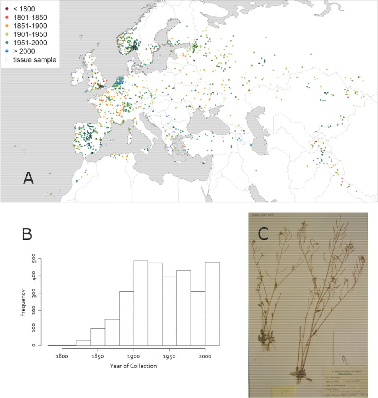
A) Locations of collections used in our analysis. Color of circle corresponds to year of collection. B) Distribution of years of collection. C) Sample herbarium record from Nepal on April 5, 1952, with a Δ13C of 21.9, a δ15N of 3.6, and a C:N ratio of 23.4.
Correlations among phenotypes
We found generally weak correlations among phenotypes of Arabidopsis individuals (Question 1). The first two principal components explained only 36.3% and 24.1%, respectively, of the variance in the five phenotypes of Δ13C, δ15N, date of collection, C:N, and PTU (N = 397). The first principal component corresponded to a negative correlation between C:N versus day of collection (bivariate r = −0.194) and PTU (bivariate r = −0.0972). Inspecting the relationship between collection date and C:N further revealed a triangle shape (Figure 2B), i.e. there were no late-collected individuals with high C:N. ANOVA showed the slopes of the regression of the 25th and 75th percentiles to be significantly different, indicating that plants with the earliest collection dates show a different relationship to C:N than later collected plants (p = 0.002, Figure S18). In a GAM where C:N was a function of date or accumulated photothermal units, we found both measures of phenology were negatively correlated with C:N across the Arabidopsis native range, but this was insignificant at the 95% confidence interval when the effect of year of collection was included (Figure S20). The second PC corresponded to a negative correlation between Δ13C and δ15N (bivariate r = −0.218). C:N and leaf proportion N are highly correlated (bivariate r = −0.815), so we focus on C:N. See supplementary material for leaf N results.

(A) Variation in phenotypes across the native range of Arabidopsis for Δ13C, δ15N, C:N, collection date, and photothermal units (PTU) at collection. Color indicates the fitted mean value of the phenotype. Collection date is earlier in the southwest and Turkey in comparison to other regions; however, PTUs are higher in the southwest and in the northeast. δ15N is variable across the range. C:N shows a gradient of increasing to the southeast and southwest. Δ13C increases along a northeasterly gradient. (B) Correlations between phenotypes in this study. There is a positive trend between PTU and date of collection. PCA of phenotypes showed an inverse relationship between C:N and PTU and an inverse relationship between Δ13C and δ15N along the first and second principal components (C). Arrows represent correlation of phenotypes with principal components. Latitude (correlation with first PC r = −0.183) and longitude (correlation with first PC r = −0.116) correlations are shown for geographic context, though they were not included in PCA.
Spatial variation in long-term average phenotypes
We visualized spatial diversity in phenotypes by plotting the intercept surfaces in the year only models (Figure 2A). All phenotypes showed significant spatial variation (all GAM smooth terms significantly different from zero). Δ13C was lower in the Iberian Peninsula and higher in Russia (GAM smooth term, p = 0.0002). δ15N varied across the range, but with less pronounced spatial gradients (GAM smooth term, p = 0.003). C:N was higher in the Iberian Peninsula and the East and lower in Russia (GAM smooth term, p = 8e-05). Collection day was earlier along the Atlantic coast and Mediterranean (GAM smooth term, p = <2e-16). Despite this, PTU at collection still was higher in the Mediterranean region as well as at far northern, continental sites (GAM smooth term, p = <2e-16).
Several phenotypes have changed significantly across large regions over the study period (1794-2010, Figure 3 above). For example, C:N ratio increased in later years in much of southwestern Europe. δ15N decreased significantly throughout most of the range. Collection date and PTUs became significantly later in many regions from the Mediterranean to Central Asia, although collection date became significantly earlier in the extreme south (Morocco and Himalayas). There was no significant temporal trend in Δ13C (not shown).

Change in phenotypes across years for collection date (A), photothermal units (B), δ nitrogen (C), and C:N (D). Color indicates the value of the coefficient for year in the model excluding climate variables, gray shading indicates regions where estimated coefficient is not significantly different from 0. Day of collection and photothermal units have significantly increased over time in most of the range, but with some exceptions for day of collection in the south. Change in collection day was uneven across regions, with greater shifts in the Aegean than in the Scandinavian Peninsula. δ15N significantly decreased across most of the range, and C:N increased, most notably in the southwest. Inset scatterplot in A shows the significant increase in collection date with year for samples in the boxed Mediterranean region. Plots to the left of A show the density of collection dates through the year remains stable through time for Scandinavian collections within the boxed region (top) but shift toward more collections late in the year in the boxed Mediterranean collections (bottom).
Temporal change in phenotypes after accounting for climate anomalies
The temporal trends in phenotypes across the study period were likely partly related to underlying climate variation. However, many of the phenotypes were still significantly associated with year of collection even when accounting for temporal anomalies in climate from 1901-2010. There was a general delay in collection through time in much of the eastern range (Figure S1, S2). However, Iberian collections were significantly earlier in later years. Across most of Europe, later years of collection also were associated with significantly greater C:N ratio (Figures S9, S10). Similarly, we observed δ15N decreasing in later years across much of Arabidopsis’ range. There was still no significant temporal trend in Δ13C.
Phenotype associations with spatiotemporal climate gradients
Date of collection
In years (temporal models) with a relatively warm January or April plants were collected significantly earlier (Figure 4A). Similarly, in locations (spatial models) with warmer temperatures plants were collected earlier, though in many regions these coefficients were non-significant. We also tested associations with July aridity index (precipitation/PET) and found that plants were collected significantly earlier in years (temporal models) with dry summers in central/eastern Europe, but later following dry summers in Central Asia (Figure 4B).

Association between collection day of Arabidopsis temporal mean April temperatures (A) and July aridity index (B) anomalies (compared to 50-year average). Color indicates the value of the coefficient of the April mean temperature or July aridity index term. In years where April was warmer, plants were collected earlier. In wetter years, plants were collected later in Eastern Europe but earlier in Asia. Shading indicates regions where estimated coefficient is not significantly different from 0. Scatterplots of phenotype measures for individuals within the boxed areas show a decreasing collection date with mean April temperature and increasing collection date with July aridity index in Eastern Europe and decreasing collection date in Central Asia.
Photothermal units
To standardize spatiotemporal variation in developmental periods, we also modeled climate associations with PTUs. There were few areas where temperature anomalies were significantly associated with PTUs (Figure S3). However, in some areas, accumulated PTUs at collection changed significantly in association with spatial temperature gradients (Figure S4). Locations with warmer Aprils had plants collected at more PTUs around the Baltic sea and fewer PTUs around the Aegean. In the temporal model, plants from Western Europe, the Aegean, and Central Asia were collected at lower PTUs in wetter years. In the spatial model, plants from wetter areas in the south were collected at lower PTUs, but this pattern was reversed in the North (Figure S3, S4).
Δ13Carbon
Wet summers were not significantly related to Δ13C in any region in either the temporal or spatial models. However, there was a significant change in the spatial relationship between Δ13C and long-term mean April temperature (smooth term significance: p = 2e-5). Specifically, in Central Asia areas with warmer Aprils had higher Δ13C than collections from areas with cooler Aprils (Figure S6A), while in Iberia and Northeastern Europe, the reverse was true (though the local relationships were not significant). Although elevation was not included in final models for reasons discussed above, replacing year with elevation in the temporal model showed a significant negative association between elevation and Δ13C (Figure S13).
δ15Nitrogen
δ15N was significantly higher in wetter years in Iberia, Asia, and Central Europe, (Figure S7), but lower in the North of France. Temperature was only significantly positively related to δ15N in the case of spatial variation in minimum January temperatures around the North Sea.
Leaf C:N
Leaf C:N was significantly different among locations (spatial models) differing in April mean temperature and January minimum temperature, although the direction of these trends differed among regions. Specifically, sites with warmer winters were associated with higher C:N in southwestern Europe but lower C:N in central Asia (Figure S10B) and sites with warmer temperatures in April predicted lower C:N in Iberia. For the temporal model, plants collected in wetter years in Iberia had significantly higher C:N ratios.
Comparison of results to hypotheses
Correspondence of hypothesized phenotype response to increases in temperature, rainfall, or year with observed model output. Green boxes indicate that temporal or spatial models supported the hypothesis, with a significant relationship within the 95% confidence interval in the proposed direction. Red boxes indicate that temporal or spatial models were either insignificant or significant in the opposite direction to the predicted trend. Blue boxes indicate that the temporal or spatial models showed a high level of regional variation, with collections in some geographic areas supporting and others contradicting the hypothesis.
Discussion
Widely distributed species often exhibit considerable phenotypic diversity, a large portion of which may be driven by adaptive plastic and evolutionary responses to environmental gradients. The existence of genetic variation in environmental responses among populations suggests that responses to temporal environmental shifts may differ dramatically among populations. Previous studies of intraspecific trait variation in response to environment have tended to focus on genetic variation of environmental responses in common gardens (e.g. Wilczek et al. 2009; Kenney et al. 2014), temporal trends in phenology from well-monitored sites (e.g. CaraDonna et al., 2014), or field sampling of individuals from a small number of sites (e.g. Jung, Violle, Mondy, Hoffmann, & Muller, 2010). Here, we complement this literature by studying change in traits across an entire species range over two centuries, giving us a window into drivers of intraspecific diversity and regional differences in global change biology. From the accumulated work of field biologists contained in natural history collections, we tested hypotheses about variation in life history and physiology in response to environment. We observed modest evidence of coordinated phenological-physiological axes of variation. We found later flowering times and higher accumulated photothermal units over the study period across most of the range and lower δ15N and higher C:N in more recent collections. Additionally, we observed distinct regional differences in phenology, Δ13C, and C:N in response to rainfall and temperature.
Intraspecific variation in life history and physiology shows little coordination along a single major axis (question 1)
We found little evidence for tight coordination among studied phenotypes, fitting with some past surveys that found weak to no support for a single major axis in intraspecific trait variation in response to environment across diverse plant growth forms (e.g. Albert et al. 2010; Wright & Sutton Grier 2012). Common garden experiments often find substantial genetic covariation between the traits we studied possibly due to pleiotropy or selection maintaining correlated variation (Des Marais et al., 2012; Kenney et al., 2014; McKay et al., 2003). By contrast, the massively complex environmental variation organisms experience in the wild may combine with genotype-by-environment interactions to generate high dimensional trait variation among individuals in nature.
Nevertheless, we found modest evidence of a life history-physiology axis: plants collected later in the year had low leaf C:N, indicative of a fast-growing resource acquisitive strategy with low investment in C for structure and high investment in N for photosynthesis. This strategy may be adaptive for rapid-cycling plants germinating and flowering within a season (spring/summer annuals), contrasted with slower-growing genotypes known to require vernalization for flowering over a winter annual habit. Indeed, Des Marais et al. (2012) found that vernalization-requiring (winter annual) Arabidopsis genotypes had lower leaf N than genotypes not requiring vernalization for flowering, the latter of which could also behave as spring or summer annuals.
The negative correlation we observed between Δ13C and δ15N has been reported by other authors and suggested to be a result of independent responses to multiple correlated environmental variables rather than an intrinsic biological limitation. Environmental variables with opposing effects on Δ13C and δ15N include soil, temperature, and rainfall patterns (Hartman & Danin, 2010; Liu et al., 2007; Peri et al., 2012), due to depletion of soil N and changes in stomatal opening, and atmospheric carbon (Bloom, Burger, Asensio, & Cousins, 2010), which increases carbon uptake while suppressing nitrate assimilation.
Arabidopsis life history and physiology vary across spatial environmental gradients, suggesting adaptive responses to long-term environmental conditions (question 2)
Geographic clines in traits in nature may be due to adaptive responses to environment; however, the spatial differences in traits or trait changes through time we observed are difficult to ascribe to genetic or plastic causes because of unknown genotype-environment interactions in the field and the confounding of environmental gradients and population genetics. The 1001 Genomes Project identified genetic clusters of Arabidopsis that were somewhat geographically structured but noted that these clusters overlapped and were distributed across a wide range of environments (Alonso-Blanco et al., 2016) (see figure S21 for a map of the clusters). We observed patterns of significant phenotype-environment relationships that spanned multiple genetic clusters and that followed our expectations for how phenology could affect fitness, while physiological traits were less clear.
Physiology, Leaf Economic Spectrum
The Leaf Economic Spectrum and fast/slow life history predictions were not well supported by our results for C:N, Δ13C, and δ15N response to climate, since we saw both positive and negative trends with temperature and aridity depending on geographical region. This may be due to the intraspecific nature of our study, as opposed to the interspecific data often used to support the LES. In multispecies analyses, phenotype correlations with climate may be influenced by community composition changes across the environment or may not represent the physiology or climate responses of individual species (Albert et al., 2010; Elmore, Craine, Nelson, & Guinn, 2017). In addition, our study may have overlooked the effects of edaphic conditions on C:N and δ15N. C:N over most of the native range was insignificantly related to spatial and temporal gradients of temperature and aridity index (July precipitation/PET) but increased with year as seen in grassland communities due to rising Ca (Gill et al., 2002). Likewise,δ15N over most of the range neither decreased with aridity index nor responded to temperature as expected, but did decrease with year as previously reported in multi-species surveys (McLauchlan et al., 2010), possibly due to CO2 enrichment.
Similarly, we did not see strong relationships between aridity index and Δ13C. Δ13C was expected to be related to rainfall and temperature due to Δ13C being a proxy for stomatal gas exchange (Diefendorf et al., 2010; Farquhar et al., 1989). There are at least three potential explanations for weak Δ13C relationships with climate. First, we observed both positive and negative trends for aridity and date of collection, consistent with the hypothesis that Arabidopsis exhibits both drought escaping and drought avoiding genotypes. The phenological response to moisture of rapid flowering (drought escape strategy) could confine growth to periods of high moisture, obviating any stomatal closure in response to soil drying (and hence no effect on Δ13C). Stated simply, phenology and physiology cannot be treated as completely independent traits. Second, variation in plant traits we did not directly consider may affect Δ13C. Gas exchange and carbon assimilation depend in part on leaf architecture and physiology traits like venation, root allocation, and mesophyll conductance (Brodribb, Feild, & Jordan, 2007; Easlon et al., 2014; Schulze, Turner, Nicolle, & Schumacher, 2006), which could limit responses in Δ13C. For example, greater investment in roots could allow plants in relatively drier conditions to maintain open stomata, preventing decreases in Ci and leading to no observed climate effect on Δ13C. Third, elevated atmospheric partial CO2 could mitigate climate effects on Δ13C by increasing the efficiency of stomatal gas exchange (Drake et al., 2017). Local investigations of the patterns we found could complement our results by characterizing the underlying ecophysiological and life history mechanisms driving intraspecific variation. For example, local studies could allow more precise measurement of environmental conditions, and could remove some of the contribution of major genetic turnover among populations (including populations referred to as relicts, Alonso-Blanco et al., 2016), that may cause unexpected regional differences in phenotype trends (Figure S1D).
Phenology
We found strong spatial gradients in two measures of phenology, suggesting that adaptive responses to climate drive long-term intraspecific phenotypic differences among regions. Locations that were warmer than average in either April or January corresponded to significantly earlier collection dates, consistent with temperature’s positive effect on growth rate (Wilczek et al., 2009). In addition, our models provided support that some phenological variation did reflect seasonality of moisture availability. We found that Arabidopsis was collected significantly earlier in years with dry summers in central Europe and at significantly lower PTU in regions of wet summers around the Mediterranean, suggesting drought escape or avoidance strategies, respectively, could be important in those regions. Alternatively, later collections in wetter years could be the result of multiple successful generations due to the extra rainfall.
Changes in Arabidopsis life history and physiology over the last two centuries track climate, suggesting adaptive responses (question 3)
Increasing global temperatures were expected to increase relative growth rate and hasten germination, decreasing flowering time as measured by collection date. In addition, atmospheric CO2 enrichment was expected to increase Δ13C (Drake et al., 2017) and C:N and decrease δ15N (Bloom et al., 2010). With increasing environmental nitrogen due to human activity (Galloway et al., 2004), we expected δ15N to decrease.
This is largely what we found in the year models for leaf physiology. Δ13C did not significantly change through time across the native range, which could be due to differential response to aridity gradients across the locations sampled (Drake et al., 2017). Geographic variation in the strength of the relationships for other traits could be due to underlying genetic variation or interaction with environmental factors we did not account for. Nevertheless, C:N increases and δ15N decreases as expected across large portions of the native range.
For collection date and PTU, however, our models returned the surprising result of later collection rather than earlier, despite earlier collections in warmer years. The fact that the relationship between warmth and collection date was spatially variable, and insignificant in some regions, may indicate areas of contrasting phenological response, perhaps due to lost vernalization signal or variable effects on germination (Burghardt, Edwards, & Donohue, 2016). Variation across space in phenological response to climate change has been shown before and may be due to genetic differences among populations or due to interactions with other environmental variables (Park et al., 2018). Alternatively, Arabidopsis is known to complete a generation within a single season, climate permitting, and warmer climates may allow for fall flowering (Fournier-Level et al., 2013; Wilczek et al., 2009). If warmer temperatures enable a greater number of spring or summer germinants to flower before winter in regions such as Central Europe, we would expect to see later collection dates in more recent years (Burghardt et al., 2015). In this case, regions that have earlier collection dates with warmer temperature may be limited in generational cycles due to another environmental factor, such as summer drought or short growing seasons.
Our findings of later collection dates through the study period (1798-2010) may surprise some readers due to previously observed acceleration of temperate spring phenology (Parmesan & Yohe, 2003). However, we modeled changes in mean phenological response to environment, which can be weakly related to either tail of phenology trait distributions (CaraDonna et al., 2014). Individuals on the extremes, such as first-flowering individuals, are often the primary focus of studies showing accelerated spring phenology in recent years. Why might Arabidopsis flower later even as global temperatures rise? First, non-climate environmental changes (e.g. shifts in land use toward human-dominated landscapes) may drive phenology by favoring spring germinants. Second, warming climate or increasing atmospheric pCO2 may favor alternate life histories by increasing relative growth rate, thus allowing spring or fall germinants to complete their life cycle before conditions degrade at the end of a growing season. Later collections in more recent years might represent an increasing proportion of fast-growing spring or summer annuals as opposed to winter annuals. Whatever the cause of Arabidopsis flowering later, these phenological changes may have important ecological effects, such as altered biotic interactions.
Our approach, technical limitations in herbaria data to surmount in future studies
Understanding how environmental variation drives the intraspecific diversity in broadly distributed species has been challenging due to logistics of large spatiotemporal scales. However, advances in digitization of museum specimens and the generation of global gridded spatiotemporal environmental data are opening a new window into large scale patterns of biodiversity. One challenge of herbarium specimens is that they typically present a single observation of a mature, reproductive individuals. Thus, these specimens contain limited information on phenology and physiology at earlier life stages (e.g. seedling plants), which can have subsequently strong impacts on later observed stages. Use of developmental models (Burghardt et al., 2015) might allow one to backcast potential developmental trajectories using herbarium specimens and climate data, to make predictions about phenology of germination and transition to flowering. In addition, herbaria collections are often biased by factors such as geography, species, and climate (Daru et al., 2018; Loiselle et al., 2008). Hierarchical sampling through repeated collections in the same region could improve the confidence of our model in representing phenotypic change through time.
Generalized additive models are a flexible approach to model phenotype responses to environment that might differ spatially among populations (MacGillivray et al., 2010). These models allow the data to inform on spatial variation in the trends studied, unlike approaches that bin individuals into discrete and arbitrarily bounded regions. Herbarium records represent imperfect and biased samples of natural populations (Daru et al., 2018), and future efforts may benefit from additional information that might allow us to account for these biases. Here, we sampled a very large number of specimens across continents and centuries, perhaps reducing the effect of biases associated with specific collectors. Nevertheless, as museum informatics advance it may become possible to explicitly model potential sources of bias, for example those arising from collecting behavior of specific researchers.
Conclusion
Widely distributed species often harbor extensive intraspecific trait diversity. Natural history collections offer a window into this diversity and in particular allow investigation of long-term responses to anthropogenic change across species ranges. Here we show that spatiotemporal climate gradients explain much of this diversity but nevertheless much of the phenotypic diversity in nature remains to be explained.
Acknowledgements
Hundreds of botanists collected the specimens studied here. The staff at herbaria at Oslo Natural History Museum, Kew Gardens, Real Jardin Botanico, Komarov Botanical Garden, the New York Botanical Garden, and the British Museum of Natural History gave permission for tissue sampling. Michelle Brown provided essential assistance in collecting herbarium tissue. Jason Bonnette helped coordinate sample preparation. Major assistance in digitizing of specimens was provided by Patrick Herné. Eugene Shakirov aided in translating Russian specimen labels. Data from the MNHN in Paris were obtained thanks to the participatory science program Les Herbonautes” (MNHN/Tela Botanica) which is part of Infrastructure Nationale e-RECOLNAT: ANR-11-INBS-0004. Additional volunteers from the Atlas of Living Australia helped with digitization and georeferencing. Funding was provided by an Earth Institute fellowship to JRL.
The authors report no commercial or other relationships relevant to the content of this article that would represent a conflict of interest.
References


