

ABSTRACT
Evolutionary relationships between species are traditionally represented in the form of a tree, called the species tree. The reconstruction of the species tree from molecular data is hindered by frequent conflicts between gene genealogies. A standard way of dealing with this issue is to postulate the existence of a unique species tree where disagreements between gene trees are explained by incomplete lineage sorting (ILS) due to random coalescences of gene lineages inside the edges of the species tree. This paradigm, known as the multi-species coalescent (MSC), is constantly violated by the ubiquitous presence of gene flow revealed by empirical studies, leading to topological incongruences of gene trees that cannot be explained by ILS alone. Here we argue that this paradigm should be revised in favor of a vision acknowledging the importance of gene flow and where gene histories shape the species tree rather than the opposite. We propose a new, plastic framework for modeling the joint evolution of gene and species lineages relaxing the hierarchy between the species tree and gene trees. We implement this framework in two mathematical models called the gene-based diversification models (GBD): 1) GBD-forward, following all evolving genomes and thus very intensive computationally and 2) GBD-backward, based on coalescent theory and thus more efficient. Each model features four parameters tuning colonization, mutation, gene flow and reproductive isolation. We propose a quick inference method based on the differences between gene trees and use it to evaluate the amount of gene flow in two empirical data-sets. We find that in these data-sets, gene tree distributions are better explained by the best fitting GBD model than by the best fitting MSC model. This work should pave the way for approaches of diversification using the richer signal contained in genomic evolutionary histories rather than in the mere species tree.
- coalescent theory
- gene flow
- gene tree
- gene-based diversification model
- multi-species coalescent
- phylogeny
- population genetics
- speciation
- species tree
- reproductive isolation
- introgression
The most widely used way of representing evolutionary relationships between contemporary species is the so-called species tree, or phylogeny. The high efficiency of statistical methods using sequence data to reconstruct species trees, hence called ‘molecular phylogenies’, led to precise dating of the nodes of these phylogenies [35, 38, 87]. Notwithstanding the debatable accuracy of these datings, the use of time-calibrated phylogenies, sometimes called ‘timetrees’ [34], has progressively overtaken a view where phylogenies merely represent tree-like relationships between species in favor of a view where the timetree is the exact reflection of the diversification process [61, 70, 85]. In this view, the nodes of the phylogeny are consequently seen as punctual speciation events where one daughter species is instantaneously ‘born’ from a mother species. In this paper, we explore an alternative view of diversification, acknowledging that speciation is a long-term process [17, 43, 72] and not invoking any notion of mother-daughter relationship between species as done in the timetree view. This alternative view is gene-based rather than species-based, comparable with Wu’s genic view of speciation [91]. We use here the term ‘gene’ in the sense of “non-recombining locus”, i.e., a region of the genome with a unique evolutionary history. Our view is meant in particular to accommodate the well-recognized existence of gene flow between incipient species, which persists during the speciation process and long after [51].
The timetree view of phylogenies does acknowledge that gene trees are not independent and may disagree with the species tree [48], but current methods jointly inferring gene trees and species tree rely on the following assumptions that we question in the next section: there is a unique species tree, the species tree shapes the gene trees and the species tree is the only factor mediating all dependences between gene trees (they are independent conditional on the species tree).
This view is materialized in a model called the ‘multispecies coalescent’ (MSC) [39] where conditional on the species tree, the evolutionary histories of genes follow independent coalescents constrained to take place within the hollow edges of the species tree. Many methods have been developed to estimate the species tree under the MSC, such as full likelihood methods (e.g. BEAST [35], BPP [94]) which average over gene trees and parameters [93], and the approximate or summary coalescent methods (e.g. ASTRAL [58], MP-EST [45], and STELLS [92]) which use a two-step approach: gene trees are first inferred and then combined to estimate the species tree that minimize conflicts among gene trees. Discordance between gene topologies is then explained, as a first approximation at least, by the intrinsic randomness of coalescences resulting in incomplete lineage sorting (ILS) (figure 1).

Gene trees and species tree conflicts. The species tree of A, B, and C is depicted in black. In pink (gene 1) and green (gene 2) are two gene trees congruent with the species tree, i.e. with A and B being sister species. In light blue (gene 3), the tree of a gene undergoing gene flow between species B and C. In dark blue (gene 4), the tree of a gene undergoing incomplete lineage sorting.
However, the presence of gene flow (introgression, hybridization, horizontal transfer) is now widely recognized between closely related species, and even between distantly related species [51]. Porous species boundaries, allowing for gene exchange because of incomplete reproductive isolation, are indeed regularly observed in diverse taxa such as amphibians [21, 68], arthropods [12], cichlids [90], cyprinids [6, 24, 25, 26, 84], insects [63, 67, 89], and even more frequently among bacteria [51, 83]. Long neglected, gene flow has recently been recognized as an important evolutionary driving force, through adaptive introgression or the formation of new hybrid taxa [1]. The ubiquity of genetic exchange across the Tree of Life between contemporary species suggests that gene flow has occurred many times in the evolutionary past, and might actually be the most important cause of discrepancies between gene histories (e.g. [8, 11, 23, 37]) (figure 1). Accordingly, several extensions to the MSC model have been considered allowing for gene flow between species [40, 95]. These models acknowledge that species boundaries can be permeable at a few specific timepoints [33]. Unfortunately, because of the heavy computational cost of modeling the coalescent with gene flow, these methods are limited to small data-sets [95]. More importantly, they might not be appropriate to realistically model gene flow, given the frequency of gene flow across time and clades described in empirical studies [82]. Additionally, some of these methods, ASTRAL and MP-EST, might infer erroneous gene trees when gene flow is present [47]. These observations urge for novel approaches where gene flow is the rule rather than the exception.
To fill this void, we propose here an alternative framework and two accompanying models (one in forward time and one in backward time), the gene-based diversification (GBD) models, framed with minimal assumptions arising from recent empirical evidence. Those models rely on the property of populations to spontaneously differentiate genetically (mutation) while simultaneously undergoing gene flow. This genetic differentiation is accompanied by a decrease in gene flow until reproductive isolation is complete (these processes are detailed below). Moreover, unlike previous models, we place ourselves in the case of pervasive gene flow among species that may have occurred countless times in the past, as suggested by recent studies. The GBD models are anchored in a new conceptual framework, that we call the genomic view of diversification. Unlike the timetree view, the present framework does not put the emphasis on the species tree (which in our model becomes a network rather than a tree) and assumes that gene trees shape the species tree (rather than the opposite).
THE GENOMIC VIEW OF DIVERSIFICATION
Gene flow and the questionable existence of a species genealogy
The biological species concept (BSC [54]) defines species as groups of interbreeding populations that are reproductively isolated from other groups. This definition postulates the non-permeability of species boundaries, which is contradicted by the growing body of evidence describing permeable or semi-permeable genomes, even between distantly related taxa. To integrate the possibility of gene flow into the definition of species, Wu [91] shifted the emphasis from isolation at the level of the whole genome to differential isolation at the gene level. Species are thus defined as differentially adapted groups for which inter-specific gene flow is allowed except for genes involved in differential adaptation (a well-defined form of divergence in which the alternative alleles have opposite fitness effects in the two groups) [91]. Because a fraction of the genome may still be exchanged after speciation is complete, a mosaic of gene genealogies is expected between divergent genomes [91]. Much evidence supports this prediction with the observation of highly conflicting gene trees, e.g. Darwin’s finches [27, 29], sympatric sticklebacks [73, 77], Iberian barbels [25], and Rhagoletis species [2].
Accordingly, the notion of a species genealogy as the binary division of species into new independently evolving lineages in bifurcating phylogenetic trees, appears inappropriate. To avoid this misleading vision of speciation, we here wish to relax the species tree constraint by considering only gene genealogies as real genealogies, thereby laying aside, at least temporarily, the notion of species genealogy. To do so, we do not specify mother-daughter relationships between species, yet we postulate the existence of species at any time, and assume that we can unambiguously follow the genealogies of genes (defined as non-recombining loci, as mentioned above).
Looking forward in time, genes belonging to two distinct individuals may find each other, in a next generation, in the same genome because of recombination. The same process might occur with two individuals belonging to different species under gene flow.
The notion of a species genealogy as a binary bifurcating tree is hardly compatible with gene flow, and a direct consequence is to challenge the notion of a unique ancestral species. If all genes ancestral to species S have travelled through the same species in the past, then species S has only one single ancestor species at any time. But because of gene flow, these genes may lie in different species living at a given time in the past, such that species S can have several ancestral species at this time. In other words, several species have contributed to the present-day genome of the species S.
Genomic coadaptation under continuous gene flow
While some genes (e.g., genes involved in divergent adaptation) are hardly exchanged between populations, other genes (e.g., neutral genes unlinked to genes under divergent selection) can be subject to gene flow between different species [69, 91]. Gene flow can persist for long periods of time, with evidence suggesting introgression events occurring over periods lasting up to 20 Myr [6, 25, 90]. Over time, genetic differences will accumulate in regions of low recombination and expand via selective sweeps, leading eventually to complete reproductive isolation [91]. Because populations differentially accumulate new alleles, their compatibility (hybrid fitness) will be affected. This process has been conceptualized by Dobzhanzky and Muller [13, 62] in the so-called Bateson-Dobzhanzky-Muller (BDM) model [10]. This model proposes that genetic incompatibilities, hence called BDM incompatibilities, are characterised by negative epistatic interactions between alleles at two or more genes that have fixed differentially, in each of the parental populations, by local adaptation or genetic drift. The selective value of hybrids is reduced because the new alleles, divergently selected in each populations, are not adapted to each other. On the other hand, in the parental populations these alleles are co-adapted and have neutral or even beneficial effects [79, 88]. These incompatibilities have been hypothesized to increase at a rate proportional to the square of time [64]. Accordingly, pairs of species will likely exhibit greater genetic incompatibility as a function of time since divergence, i.e. be less permeable to gene flow, as has been observed for Iberian barbels [25], pea aphids [67], or salamanders [68]. In other words, gene lineages remaining too long isolated within different species decrease their ability to introgress the genome of the other, a property that we name genomic coadaptation and which is the consequence of spontaneous mutation.
The gene-based diversification (GBD) models
We propose here a new plastic framework, derived from the genomic view of diversification described above, that acknowledges the importance of gene flow and relaxes the hierarchy between the species tree and gene trees. We built two models, one in forward time that follows the standard view of the main biological processes responsible for diversification under gene flow, and one in backward time, less computationally intensive, with matching backward parameters (figure 2). These models that we named the gene-based diversification (GBD-forward and GBD-backward) models, use coalescent theory for modelling the joint evolution of gene and species lineages, reconciling phylogenomics with our current knowledge of species diversification. The biological mechanisms first, then the corresponding parameters, are detailed thereafter for each model.

The gene-based diversification (GBD) models. Gene genealogies through species (or populations, depending on the point of view, retrospective vs prospective) are depicted for two present-day genomes (N = 2 at t = 0) and five homologous genes (n = 5). Each grey ellipse represents a species (A-F). The grey lines represent the gene genealogies of non-sampled species at t = 0. The model assumes that species are quasi-static in the timescale of a few generations, and each species lineage is located in a separate column. The genealogies of genes depend on four processes: introgression (gene flow), mutation (non-homologous attraction), colonization (homologous attraction), and genetic drift (coalescence).

Genealogies of a single genome generated with the GBD-forward (A) and GBD-backward models (B). The labels/locations of species (or populations, depending on the point of view, retrospective vs prospective) are neutral. A) Parameter settings: α = 0.5, β = 1, δ = 0.2, n = 5 and N = 30. B) Parameter settings: a = 1, b = 0.1, d = 2, n = 5 and N = 10.

Comparison of the parameters of the GBD models. The Kullback-Leibler (KL) divergence was minimized between the distributions of BHV pairwise distances of GBD-forward and GBD-backward trees (with N = 6 and n = 10). The GBD-forward model was stopped when the number of populations was 30. Trees were built from the first 6 genomes (populations). Parameter settings: α = 0.5, β = 0.01, 0.02 and 0.05, δ ∈ [0.01, 0.04], every 0.01, n = 10 and K = 30. For each set of parameters, 6 replicates were performed and averaged. For the GBD-backward model we varied two parameters, a and b, and fixed d = 1 and c = 200. The number of time units t was set to 5, 000. We performed 15 replicates under each parameter combination in a grid of  with
with  , every 0.2, and b ∈ [0.01, 0.12], every 0.01.
The GBD-forward model
The GBD-forward model describes the joint action of four processes affecting the diversification of genomes (see figure 2): colonization, mutation, drift and introgression.
We consider a stochastically varying number of populations, all populated with individual genomes. We neglect extinctions and focus on colonization events, at which one population seeds a daughter population founded by one or several of its individuals. Genes independently accumulate mutations with time, under the infinite-allele model assumption. Mutations can be fixed or lost due to selection and genetic drift, that we summarize here under the term drift.
As a result of mutations and drift, populations differentiate genetically through time, which results in the decrease of gene flow. To model this, we follow what we term the co-adaptation between non-homologous genes and assume that introgression is governed by the numbers of co-adapted alleles in the receiver and donor populations. Right after colonization, all the genes of the daughter and mother populations carry the same alleles and so are co-adapted. Now an allele having arisen at time t by mutation on some gene is co-adapted only with the alleles carried by its genome at time t. This assumption underlies the well-known model of BDM incompatibilities described previously. Each time a mutation occurs the number of co-adapted genes among populations will decrease, reducing in turn the possibility of genetic exchange between populations.
Two populations that are completely differentiated, in the sense that all pairs of non-homologous alleles sampled from each of them are not co-adapted, can no longer exchange genes and can thus be seen as different species. Because populations are constantly differentiating from each other, we name populations in the prospective point of view (GBD-forward) what will become species only from a retrospective point of view (GBD-backward).
Demographic events are assumed to be much faster than other processes. In the time scale considered here, (1) the fixation of alleles within populations is instantaneous so that all genomes in a population are identical (we thus do not model the co-existence of several different homologous alleles within a population) and (2) a colonization event can be seen as the instantaneous replication of one population into two, actually because of (1), of one genome into two.
Parametrization
At t = 0, we consider a single monomorphic population, summarized into a single genome harboring n genes. During the diversification process, the genome of this population (n genes) will be replicated, mutations will be differentially fixed in each population, and the genomes of these populations can be replicated again. We follow the lineages of these n genes in forward time, assuming a time-discrete Markov chain associated to the time-continuous chain with the following rates.
Mutation (rate α). At any time t, each gene lineage in each population can acquire a new allele (infinite-allele model) at rate α. By definition, a new allele occurring at gene L on genome G is co-adapted with the allele present at a gene L′, for any L′ (different of L) of genome G. On the contrary, a mutation arising at gene L of genome G and a mutation arising at gene L′ of genome G′ are not co-adapted.
Colonization (rate β). At any time t, each population can be replicated at rate β into a new population which will evolve independently in the future. The newborn population is assumed to carry the same genome as carried by the mother population.
Genetic drift (rate γ). Each population undergoes Moran-type births and deaths at rate γ. In this work, we assume γ to be much larger than all other parameters, so that each population is actually monomorphic at all times.
Introgression (rate δ). At any time t, each gene lineage at locus L on genome G can be replicated and introgress genome G′ at rate δ(n - 1), proportional to the number of non-homologous loci in genome G′. If accepted by the target genome G′, the replicated lineage replaces its homologous gene lineage (at locus L in G′). The introgression is accepted with a probability equal to the fraction of the n - 1 non-homologous genes on G′ carrying an allele co-adapted with the allele carried by L.
Diversification occurs until a number K of different populations is reached and the whole process is stopped when the K populations are genetically isolated, that is, when no pair of alleles carried by different genomes is co-adapted (i.e., when all probabilities of introgression are equal to 0).
This framework can be made more complex by letting the parameters depend on time, on the gene, or on any prescribed category of genes.
The GBD-backward model
The GBD-backward model is not the exact backward picture of the GBD-forward model but relies on the same idea that genomes in different populations tend to diverge with time until they cannot exchange alleles. The consequence of this fact is that genes sampled in the same genome today will tend to be found in the same population in the past more often than by chance. We model this phenomenon by saying that the ancestral lineages of genes sampled in the same present-day genome are co-adapted, and that co-adapted genes are attracted towards each other. The GBD-backward model describes the joint action of four processes (see figure 2): non-homologous attraction, homologous attraction, coalescence and gene flow.
As explained above, in the retrospective point of view (GBD-backward), we name species the populations in which the ancestral gene lineages travel.
When two homologous gene lineages are in the same species they can coalesce when finding their common ancestor, that is merge into a single lineage (hence within the same genome).
Each gene lineage can move from its species to another species. This happens as a result of homologous attraction, non-homologous attraction and gene flow. As explained previously, (non-homologous) co-adapted genes move into the same species as a result of non-homologous attraction, which can be viewed as the backward consequence of mutations. Homologous gene lineages move into the same species as a result of homologous attraction, which can be viewed as the backward picture of a colonization event, when populations and their genomes have been replicated. Last, any gene lineage can move from its species by gene flow to an empty species, i.e., a species containing no other gene lineage ancestral to the sample.
Note that after coalescence of two homologous lineages, the resulting lineage is now ancestral to at least two genomes and thus co-adapted with all gene lineages ancestral to these genomes. As a consequence of the mere non-homologous attraction, going further back in time, all other genes will then move to the same species and further coalesce, until all homologous gene lineages have coalesced.
Equivalently to the drift process in forward time, we will assume that the coalescences are fast, so that in backward time homologous attraction events are immediately followed by coalescence of the two gene lineages.
Parameterization
At t = 0, n homologous genes are sampled in each of N distinct species. Retrospectively, the genomes of these N species (harbouring each n genes) will merge progressively in one genome of n genes at some time t in the past. Homologous genes, one by one, will merge (homologous attraction and coalescence). Merged genes will then attract all the genes of their original genomes (non-homologous attraction), until the coalescence of all homologous genes. We follow the lineages of these n genes in backward time, assuming a time-discrete Markov chain associated to the time-continuous chain with the following rates.
Non-homologous attraction (rate a). At any time t in the past, as a backward picture of genomic coadaptation, each gene lineage L escapes from its species S at rate a(n - 1) per target species S′, proportional to the number of non-homologous loci in the genome G′ hosted by S′. It is accepted in S′ based on its co-adaptation with G′. Recall that if G0 denotes the genome harboring the descendant lineage of L at time t = 0, then all gene lineages harbored by G′ that are ancestral to G0 are said co-adapted with L. Then L is accepted in S′ with a probability proportional to the fraction of the n-1 non-homologous loci of G′ that are co-adapted with it. The parameter a corresponds to the mutation parameter α of the GBD-forward model.
Homologous attraction (rate b). At any time t in the past, each gene lineage at rate b per homologous gene lineage, moves to the species harboring this homologous lineage (or in an alternative, more specific version of the model, each gene lineage belonging to some previously prescribed category, like genes contributing to reproductive isolation). This parameter corresponds to the diversification parameter β of the GBD-forward model.
Coalescence (rate c). At any time t in the past, each pair of homologous genes lying within the same species coalesces at rate c. This parameter corresponds to the genetic drift parameter γ of the GBD-forward model.
Gene flow (rate d). At any time t in the past, as a backward picture of introgression, each gene lineage escapes from its genome at rate d and enters an empty species (also called ghost species, i.e., harboring no other gene lineage ancestral to the samples, figure 2). This parameter corresponds to the introgression parameter δ of the GBD-forward model. To model the introgression of bigger chunks of DNA, we could alternatively assume that instead of one lineage, a given fraction of the lineages of a genome can simultaneously move to an otherwise empty species. We will not consider this possibility in the present work.
We define the number of ancestral species of a given genome at time t, as the number of species at time t containing gene lineages ancestral to this genome. We considered a time unit to be equal to the time elapsed between two events that we assumed to be constant for the sake of simplicity. In this manuscript we wish to explore the impact of gene flow rather than ILS to explain gene tree conflicts, and thus consider a large c value (coalescence rate) so that coalescence events are instantaneous, which is consistent with the large γ value of the forward model. Therefore, only the parameters a, b, and d have an influence on the gene genealogies in the GBD-backward model.
The GBD models were implemented in R (https://www.r-project.org) and evaluated under different sets of parameters. Because the GBD-forward model is computationally prohibitive, while giving comparable results with the GBD-backward model, we conducted most of the analyses and the inferences with the GBD-backward model. We provide a preliminary, ABC-like inference method by minimizing the difference (Kullback-Leibler divergence) between the distributions of Billera-Holmes-Vogtmann (BHV) distances (pairwise distances between gene trees) [3] in empirical vs simulated data. We applied this inference method to two empirical multi-locus data-sets showing complex evolutionary patterns due to gene flow, each comprising six morphologically and ecologically distinct species, the Ursinae (a bear subfamily) [42] and the Geospiza clade (a genus of Darwin’s finches) [20]. We estimated in particular 1) the relative amount of gene flow that has shaped each data-set, and 2) the corresponding average number of ancestral species.
MATERIAL AND METHODS
Inference method for the GBD-models
When considering several sampled genomes all containing n genes, a set of n gene trees is obtained for each particular parameter setting and each realization of the model. To characterize a set of gene trees, we employed a multidimensional summary statistic defined as the distribution of pairwise distances between gene trees. Because the GBD-models are time oriented, a tree metric for rooted trees was necessary. Among this class of metrics, those accounting only for topology (such as the Robinson–Foulds metric [71]) reached a plateau for large amounts of gene flow because the maximal distance among all pairs of gene trees was reached (results not shown). For these reasons we opted for the Billera-Holmes-Vogtmann (BHV) metric [3] that accounts for both branch lengths and topological differences, allowing us to distinguish sets of gene trees even when simulated with much gene flow. This metric is based on a view of tree space as a quadrant complex with quadrants sharing faces. Two trees with the same topology lie in the same quadrant, otherwise they lie in two distinct quadrants. At a common edge between two quadrants, the incongruent internal branches between trees have lengths equal to zero. Then a distance can be calculated between two rooted trees as the shortest path across these interconnected quadrants.
BHV distances do not rely only on the topology but also on branch lengths. The difference in topology is weighted by the branch lengths supporting these topologies, therefore uncertainties causing polytomies (or a branching pattern close to a polytomy) in gene trees will only marginally affect our results.
To compare trees that did not evolve on the same time scale, BHV distances were computed on re-scaled trees. For each set of gene trees issued from a single simulation or data-set, we rescaled all the trees so that the median of the most recent node depth is 1.
To find the best set of parameter  s, for empirical or test (simulated) trees, we employed the Kullback-Leibler (KL) divergence (package ‘FNN’ in R) as a distance metric by minimizing this distance between the distributions of BHV pairwise distances of empirical, and test trees, with simulated trees. The lower the KL divergence is the better is the fit.
Inference method accuracy
We tested the accuracy or our inference method, minimization of the difference (KL divergence) between the distributions of BHV distances, on 8 simulated data sets (test trees). Using the GBD-backward model, we built gene trees for 8 sampled combination parameters  with
with  every 0.2, and b ∈ [0.01, 0.12], every 0.01. the other parameters were fixed, d = 1, c = 200, n = 10 and N = 6. The number of time units t was set to 5, 000, which guarantees the coalescence of all homologous genes. We performed 15 replicates.
We next optimized the GBD-backward model for N = 6 and n = 10 by varying two parameters, a and b, and fixing d = 1 and c = 200. The number of time units t was set to 5, 000. We performed 15 replicates under each parameter combination in a grid of  with
with  , every 0.2, and b ∈ [0.01, 0.12], every 0.01. The parameters
  of the test trees were inferred by minimizing the KL distance between the test trees and the simulated trees from the grid.
Comparison of the GBD-models
To visually compare the reconstructed genealogies obtained with the GBD-forward and the GBD-backward model we performed simulations for genomes containing n = 5 genes, with α = 0.5, β = 1, δ = 0.2 and K = 30 for the GBD-forward, and a = 1, b = 0.1, d = 2 and N = 10 for GBD-backward model.
Next, we used our inference method (minimization of the KL distances between distributions of BHV pairwise distances) to compare the parameters of the two GBD models. We simulated the GBD-forward model with the following parameters: α = 0.5, β = 0.01, 0.02 and 0.05, δ ∈ [0.01, 0.04], every 0.01, n = 10 and K = 30. For each set of parameters, 6 replicates were performed and averaged. The simulations were stopped when the number of populations reached K = 30, and the trees were built from the first N = 6 genomes (populations). The KL distances were then minimized between the distributions of BHV pairwise distances of the GBD-forward trees and the inference grid obtained from the GBD-backward model and described in the previous section.
In order to compare the GBD-forward and GBD-backward trees, we only took into account the colonization and introgression events affecting the N = 6 genomes when reconstructing the GBD-forward trees. Indeed in forward time, all the genomes (here K = 30) are simulated with all the corresponding events affecting their genes (mutation, colonization and introgression). In backward time the events for only N = 6 genomes are simulated. Moreover in backward time mutations are not modeled, whereas in forward time each new mutation corresponds to a distinct event.
Both models gave qualitatively similar results (see the results section). However because the GBD-forward model was computationally prohibitive, all the following analyses were performed with the GBD-backward model. A simulation, with N = 6 (K = 30 for the GBD-forward to be able to reconstruct genealogies of N = 6 genomes), n = 10, a/α = 1, b/β = 1, c = 200 and d/δ = 1, took about 10 hours for the GBD-forward model and 10 minutes for GBD-backward model (Intel(R) Core(TM) i7-6700 CPU).
A single sampled genome (GBD-backward model)
We aimed to evaluate the variation in the number of ancestral species with gene flow. We performed simulations for a single sampled genome containing n genes (with n = 20, 50, 100, 200), and varied the relative amount of introgression (gene flow) compared to genetic differentiation (non-homologous attraction), ratio  (with a = 1 and d ∈ [0.2, 2], every 0.2). The number of time units t was set to 10, 000. We sampled the number of ancestral species every 500 time units starting at time t = 5, 000, and averaged these 11 values for each simulation. For each set of parameters, 5 replicates were performed and averaged.
A model is said to be sampling consistent if the same outcome is expected for any k sampled genes independently of the total number n of genes in the genome. To evaluate the validity of this property, we randomly sampled k = 20 genes from each genome of n ≥ 20 genes and computed their average number of ancestral species.
A sample of several genomes (GBD-backward model)
We evaluated the influence of the number n of genes (with n = 5, 10, 20), of the number of species N (with N = 6, 10), and of the relative amount of gene flow  (with d =1 and
  on gene tree diversity (BHV distances) (figure 6A). The other parameters were fixed, with b = 0.05 and c = 200.

Evaluation of the GBD-backward model for a single sampled genome with n genes. Parameter settings: a = 1, d ∈ [0.2, 2], every 0.2, and n = 20, 50, 100, and 200. The number of time units t was set to 10, 000. We sampled the number of ancestral species every 500 time units starting at time t = 5, 000, and averaged them for each simulation. For each set of parameters, 5 replicates were performed and averaged. A) Number of ancestral species depending on the number of genes n and on the ratio  , for one sampled genome. B) To assess the sampling consistency of our models, k lineages were randomly sampled. The number of ancestral species reported is the number of ancestral species of these k genes only.

Billera-Holmes-Vogtmann (BHV) distances among sets of gene trees simulated under the gene-based diversification (GBD-backward) model. For each set of parameters, 15 simulations were performed (with t = 5, 000, enough to reach the coalescence of all homologous genes) and the median BHV distances were calculated. A) Influence of the number of genes n (with n = 5, 10, and 20), of the number of species N (with N = 6 and 10), and of the ratio  on the BHV distances. Parameter settings: b = 0.05, d = 1, c = 200, and
  . B) Influence of the homologous attraction rate b and of the ratio
  on the BHV distances. Parameter settings: n = 10, N = 6, b = 0.01, 0.02, 0.05, 0.12, d = 1, c = 200, and
  .
.
For the same values of  and c, and for n = 10, N = 6, we also evaluated the influence of the homologous attraction rate b (with b = 0.01, 0.02, 0.05, 0.12) on gene tree diversity (BHV distances) (figure 6B).
The GBD-backward model versus the MSC model
To evaluate the ability of MSC methods to deal with gene flow, we estimated a species tree and its gene trees (MSC model with no gene flow) using sequences corresponding to gene trees simulated under the GBD-backward model (with gene flow).
A set of 10 gene trees was simulated under the GBD-backward model (with  , and d = 1) (figure 7). We simulated DNA sequences (package ‘PhyloSim’ in R [80]) corresponding to each of the 10 gene trees with model of DNA evolution estimated by modeltest (function ‘modelTest’, package ‘phangorn’ in R [76]) for the TRAPPC10 intron of the bear data-set detailed below [42]: HKY model, rate matrix: A = 1.00, B = 5.29, C = 1.00, D = 1.00, E = 5.29, F = 1.00, base frequencies: 0.26, 0.19, 0.21, 0.34. Prior to simulating the sequences, the 10 gene trees were scaled to the TRAPP10 intron phylogenetic tree length (built with RaXML 8.1.11 [86] assuming GTR (general time reversible) model with 1,000 bootstrap replicates).

Bayesian phylogenetic reconstruction from simulated sequences under the GBD-backward model. We simulated 10 gene trees for 6 species under the GBD-backward model (with  and
and  ). The Bayesian phylogenetic analysis was performed with the program BEAST. The edges of the species tree (Bayesian analysis) are depicted by pipes in light gray. PP: posterior probabilities.
The species tree and the gene trees associated were estimated from the simulated sequences with the program BEAST v. 2.4.8 [5] with the following parameters: unlinked substitution models, unlinked clock models, unlinked trees, HKY substitution model for each of the 10 genes, strict clock, Yule process to model speciation events, and 80 million generations with sampling every 5000 generations. To set the calibration time of the root we assumed that 1 time unit corresponded to 10 ky; on average the last coalescence event among the 10 GBD-backward trees occurred at t = 700. Accordingly, we used a normal distribution prior for the root heights (mean=7.0 (My); stdev=1.0).
Inference from empirical data-sets
Empirical data-sets
To evaluate if the GBD-backward model correctly reproduces the signal left by gene flow in gene trees we simulated gene trees under the GBD-backward model and under the MSC model. The adequacy between the simulated trees and empirical gene trees was estimated by comparing the distributions of pairwise gene tree distances of simulated vs empirical data-sets. The empirical clades have been chosen for their moderate phylogenetic depth, good sampling coverage and known conflicting gene trees. The first data-set comprised 14 autosomal introns for 6 bear species (Helarctos malayanus, Melursus ursinus, Ursus americanus, U. arctos, U. maritimus, and U. thibetanus) and 2 outgroups (Ailuropoda melanoleuca and Tremarctos ornatus) [42]. The sequences were downloaded from GenBank (supplementary table S1). As in Kutschera et al. [42], all variation within and among individuals was collapsed into one single 50% majority-rule-consensus sequence for each of the 8 species. The phylogenetic trees were built with the program BEAST v. 1.8.3. [14], with the parameters used by the authors of [42]: Yule prior to model the branching process, strict clock, a normal prior on substitution rates (0.001 ± 0.001) (mean ± SD), minimum age of 11.6 My for the divergence of A. melanoleuca from other bears (exponential prior: mean= 0.5; offset= 11.6), and 10 million generations with sampling every 1000 generations. The models of DNA evolution were estimated by modeltest (function ‘modelTest’, package ‘phangorn’ in R [76]) (supplementary table S2). The monophyly of the ingroup and the topology among the outgroups were constrained according to the topology depicted in Kutschera et al. [42].
The second data-set comprised 7 nuclear markers for 6 finch species (Geospiza conirostris, G. fortis, G. fulginosa, G. magnirostris, G.scandens, and G. septentrionalis) and 2 outgroups (Ca- marhynchus psittacula and Platyspiza crassirostris) [20]. The sequences were downloaded from GenBank (supplementary table S3). The phylogenetic trees were built with the program BEAST v. [14] with the parameters used by Farrington et al. [20]: coalescent constant size prior to model the branching process, strict clock, substitution rate equal to 1, specific models of DNA evolution defined by the authors (supplementary table S2), and 10 million generations with sampling every 1000 generations. The monophyly of the ingroup and the topology among the outgroups were constrained according to the topology depicted in [20].
Estimation of parameters under the multi-species coalescent (MSC) model
We optimized the MSC model for N = 6 species by varying two parameters, the speciation rate λ and the extinction rate µ, and fixing the coalescence rate to 1. Birth-death trees of 6 tips (function ‘sim.bdtree’, package ‘geiger’ in R) were simulated in a grid of (λ, µ = mλ) with λ ∈ [0.02, 0.34], every 0.02, and m ∈ [0.1, 0.65], every 0.05. Because we simulated small trees (6 tips), the degree of variation between trees simulated with the same parameters was high. Therefore for each value of (λ, µ) we randomly selected 15 species trees for which the crown age did not differ by more than 2.5% from the expected crown age. Next, we simulated 10 gene genealogies for each species tree (coalescence rate fixed to 1).
If the diversification rate (speciation rate minus extinction rate) is low, all the homologous genes will coalesce before the next node in the species tree, so that all the gene trees will have the same topology. On the contrary, if the diversification rate is too fast, some homologous genes will not have time to coalesce before the next node of the species tree, resulting in incongruent gene trees due to the randomness of coalescences (ILS).
Estimation of parameters under the gene-based diversification (GBD-backward) model
Equivalently, we optimized the GBD-backward model for N = 6 by varying two parameters, here a and b, and fixing d = 1 and c = 200 (recall c is given a sufficiently large value that coalescences are instantaneous). Since increasing n has no effect on BHV distances (see results and figure 6), we simulated genomes with n = 10 genes. The number of time units t was set to 5, 000, which guarantees the coalescence of all homologous genes. We performed 15 replicates under each parameter combination in a grid of  with
with  , every 0.2, and b ∈ [0.01, 0.12], every 0.01.
For both models (MSC and GBD-backward) we employed the Kullback-Leibler (KL) divergence (package ‘FNN’ in R) as a distance metric to find the best set of parameters by minimizing this distance between the distributions of BHV pairwise distances of empirical and simulated trees. The lower the KL divergence is the better is the fit.
RESULTS
Inference method accuracy
Using simulated data-sets, we showed that our inference method was able to give reliable estimates of simulated parameters despite its simplicity (supplementary figure 1). Even if the exact parameter combination was retrieved only twice over eight (test data sets d and e), the inferred parameters were very close to the simulated ones. We calculated the mean squared error (MSE), defined as the average squared difference between the observed (inferred parameters) and predicted values (simulated parameters). We found a MSE of 1.5e-04 for the parameter  and a MSE of 0.15 for the parameter b. This simple inference method is sufficient to estimate the parameters of the model having supposedly shaped the gene trees of the data set. More subtle methods will be developed in the future to account for more complex features, such as differential gene flow depending on putative gene categories, and to infer the very history of the embedding of gene lineages into species.
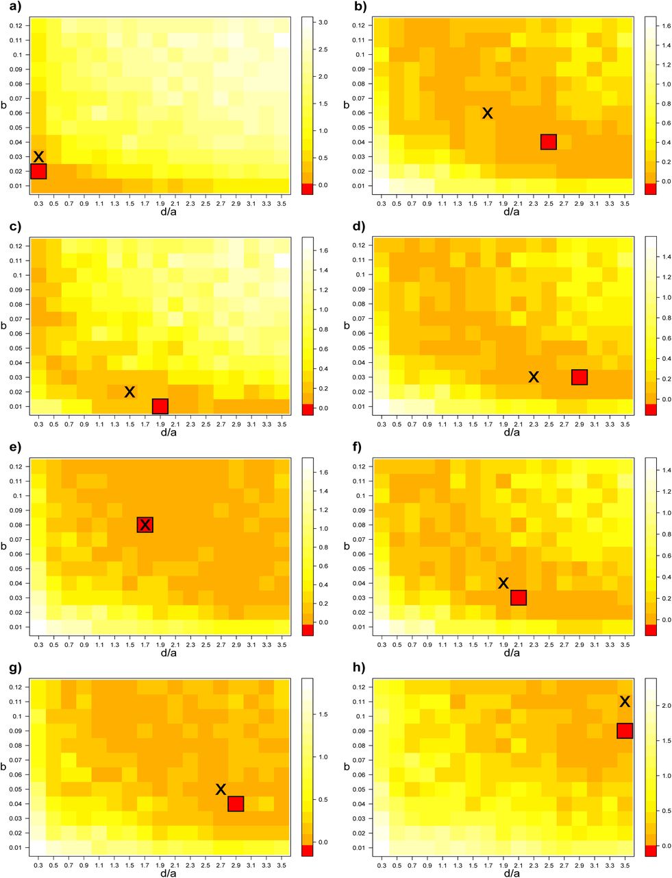
We tested our inference method, minimization of the difference (KL divergence) between the distributions of BHV distances, on 8 simulated data sets (test data sets) with 15 replicates each. For each optimization analysis, the cell for which we found the best fit between the test trees and simulated trees (smallest KL divergence) is framed. The cross indicates the combination parameters of the test data set.
Comparison of the GBD-models
Even if the two models, GBD-forward and GBD-backward, are only approximately equal, they showed a qualitatively similar pattern in gene genealogies and in dissimilarity among gene trees with increasing gene flow (figure 3 and 4). Because they are co-adapted, genes sampled in the same species at present time should have spent time together in the same species more often than by chance in the past. This property was indeed observed in both models, with genes sampled at present time frequently found together in the same species in the past (figure 3).
Using our inference method, we found a strong correlation betwee  (GBD-backward) and
  (GBD-forward) for β = 0.05 (r = 0.99 and p.value = 0.005) and β = 0.02 (r = 0.97 and p.value = 0.03). For β = 0.01 we found a high correlation but not significant correlation (presumably due to small sample size) (r = 0.89 and p.value = 0.1). Our inference method was unable to provide a good estimate for β, this estimate oscillated between 0.01 and 0.02 regardless of β. However we found a more pronounced slope for higher β indicating higher gene flow. If the colonization is fast, the number of mutations differentially acquired within each population will be small, therefore introgression events (gene flow) will be very likely among populations. With this inference method, the inclination of the slope expresses the difference in β (colonization rate).
A single sampled genome (GBD-backward)
With N = 1 sampled genome containing n genes, we let A(t) = (A1(t), …, An(t)) denote the sorting of genes into ancestral species t units of time before the present. More precisely, Ak(t) denotes the number of ancestral species containing k gene lineages, so that  and
and  is the total number of species at t ancestral to the sampled genome. For each ε ∈ (0, 1], we will also be interested in the number
  of ancestral species containing at least a fraction ε of the genome (with [x] denoting the smallest integer larger than x). All stationary quantities will be denoted by the same symbols, replacing t with ∞.
We will call a block at (backward) time t a (maximal) set of gene lineages that lie in the same species at time t. The transition rates can be specified as follows in terms of the configuration of gene lineages into blocks (i.e., ancestral species). For each pair of blocks containing (j, k) lineages, non-homologous attraction occurs at rate ajk and results in the configuration (j - 1, k + 1). For each block containing j lineages, gene flow occurs at rate dj and results in the block losing one lineage; simultaneously a new block containing 1 single lineage is created. These are exactly the same rates as in the well-known Moran model with mutation under the infinite-allele model [59], replacing ‘block’ with ‘allele’, ‘connection’ by ‘resampling’ (simultaneous birth from one of the j carriers of a given allele and death of one of the k carriers of another given allele) and ‘gene flow’ with ‘mutation’ (mutation appearing in one of the j carriers of a given allele into a new allele never existing before). For this Moran model,
the total population size is n;
at rate a for each oriented pair of individuals independently, the first individual of the pair gives birth to a copy of herself and the second individual of the pair is simultaneously killed;
mutation occurs at rate d independently in each individual lineage.
As a consequence, A(t) has the same distribution as the allele frequency spectrum in the Moran model with total population size n, resampling rate a and mutation rate d, starting at time t = 0 from a population of clonal individuals (one single block). In particular, the distribution of A(∞) is the stationary distribution of the allele frequency spectrum, which is known to be given by Ewens’ sampling formula with scaled mutation rate d/a [15, 18, 19]. Expectations of this distribution are:
 so that
 And
And
 In particular, as n → ∞,
 At stationarity, and particularly for large values of
  , the mean number of ancestral species S(∞) obtained from simulations was equal to the mathematical prediction (figure 5A). In particular, the mean number of ancestral species at stationarity increases with
  .
.
An additional key feature of this model is sampling consistency. In words, the history of a sample of k genes taken from a genome of n genes does not depend on n. This property can again be deduced from the representation of our model in terms of the better known Moran model. Indeed, the dynamics of a sample of k individuals in the Moran model does not depend on the population size, as can be seen from the so-called lookdown construction [16]. The simulations performed with k genes randomly sampled from each genome of n genes, are in agreement with this claim of sampling consistency: the number of ancestral species at stationarity 𝔼(Sε(∞)) is independent of the number of genes n (figure 5B).
A sample of several genomes (GBD-backward)
Using simulations, we evaluated the GBD-backward model for several sampled genomes (N > 1) under several combinations of parameters. As expected gene tree diversity, measured by BHV distances, increased with  , i.e. the relative amount of gene flow, and with the number of species N. Conversely our results showed that the number of genes n had no effect on distances (figure 6A). This last result, the lack of influence of n on gene tree diversity, is of particular interest, because one usually has only access to a fraction of a genome. It shows that regardless of the number of genes sampled, the resulting gene tree diversity will remain the same as long as gene trees have been shaped by processes with similar parameter values.
Our results also showed that as the homologous attraction rate b decreases, and for the same  , gene trees were more similar (lower BHV distances) (figure 6B). When a long period of time elapses between two homologous attraction events (low b), all the genes belonging to the two genomes that have started to coalesce, have enough time to converge toward the same species, and thus coalesce before the next homologous attraction event, in spite of gene flow.
GBD versus MSC: ignoring gene flow may lead to mistaken phylogenetic inferences
When evaluating the ability of MSC model to deal with gene flow, we found a strong support (posterior probabilities > 0.90) for all the nodes of the Bayesian species tree even if the individual gene trees of the GBD-backward model did not corroborate this topology (figure 7). For example, 7 out of 10 gene trees modeled under the GBD-backward model support the connection between species E and species C and D, and only 3 the direct relationship between species E and F. On the contrary, the Bayesian tree strongly supports the clade (E,F) with a posterior probability equal to 1, and considers all the connections between E and (C,D) to be due to ancestral polymorphism (i.e., ILS). Moreover because gene trees are constrained in the species tree (MSC model), the coalescences between genes of E and (C,D) must take place after the species tree coalescence, therefore these coalescences are timed around 7 My instead of 2 My according to the GBD-backward tree. Failing to recognize that gene flow may have shaped gene genealogies, hence DNA sequences, can result in important topological and dating errors.
The GBD-backward model correctly captures the signal left by gene flow in empirical data-sets
To find the best set of parameters, we minimized the Kullback-Leibler (KL) divergence between the distributions of BHV pairwise distances of empirical and simulated trees (figure 8). Under the multi-species coalescent (MSC) model, the most likely set of parameters was µ = 0.4 × λ and λ = 0.2 (KL divergence = 0.23) for the bears, and µ = 0.45 × λ and λ = 0.22 for the finches (KL divergenc = 0.12). We noted longer tailed distributions for the distances between trees modeled under the MSC model than for the empirical data-sets (figure 9). This skewed distribution obtained with the MSC model explains why we did not detect a sharp peak in the optimization landscape for the MSC model (figure 8).

Minimization of the Kullback-Leibler (KL) divergence between empirical and simulated trees, i.e. between their distributions of BHV pairwise distances. Two parameters were optimized for each model. The speciation rate (λ) and the extinction rate (µ) for the multi-species coalescent (MSC) model (with coalescence rate set to 1). The homologous attraction b and the ratio of the gene flow rate over the non-homologous attraction rate  for the gene-based diversification (GBD-backward) model (with d set to 1). For each set of variables, 15 simulations were performed and averaged. The same color scale was used for each empirical data-set. For each optimization analysis, the cell for which we found the best fit between empirical and simulated trees (smallest KL divergence) is framed.

Best fit between empirical and simulated trees, i.e. between their distributions of BHV pairwise distances (selected cells of figure 8). For each set of variables, 15 simulations were performed and averaged. a: non-homologous attraction rate, b: homologous attraction rate, d: gene flow rate (set to 1), λ: speciation rate, µ: extinction rate, KL: Kullback-Leibler.
Under the gene-based diversification (GBD-backward) model, the most likely set of parameters was b = 0.03 and  (KL divergence = 0.14) for the bears, and b = 0.11 and
  for the finches (KL divergence = 0.01) (figure 8). Contrary to the MSC model, the distributions of the distances between trees modeled under the GBD-backward model or empirical trees did not show, or to a lesser degree, a long tail (figure 9), explaining why we could detect a sharp peak in the optimization landscape for the MSC model (figure 8).
Comparing the parameters λ and µ to b and  is not straightforward as the two models, MSC and GBD-backward, are built under different assumptions. However in both cases, the parameters influence the diversity among trees (shape of the distribution of BHV pairwise distances). A greater diversity among trees is expected with increasing λ and decreasing µ, and with increasing
  and b, allowing us to explore the parameter landscape to find the setting that minimizes the distance between simulations and empirical data-sets for each model.
Given our results and the mathematical predictions, the time-averaged number Sε(∞) of ancestral species to the sampled genome containing at least 10% of the genome (ε = 0.1) when n → ∞ is 4.8 for the bear data-set and 3.4 for the finch data-set.
DISCUSSION
Within species, gene flow allows the maintenance of species cohesion in the face of genetic differentiation [60, 81], preventing genetic isolation of populations and the subsequent emergence of reproductive barriers leading to speciation [10]. Among species, the existence of gene flow challenges the notion of a species genealogy as well as the current concepts of species. Indeed, if gene flow is as pervasive as recent empirical studies suggest [8, 11, 23, 37], the genealogical history of species should be represented as a phylogenetic network encompassing the mosaic of gene genealogies. Similarly, it seems very conservative to delineate species based on the widely used biological species concept (reproductive isolation) [54], or phylogenetic species concept (reciprocal monophyly) [65]. Because of the ubiquity of gene flow, which can persist for several millions of years after the lineages have started to diverge (i.e., onset of speciation) [4, 49], species should be rather defined by their capacity to coexist without fusion in spite of gene flow [50, 74].
The simplified view of diversification, consisting in representing lineages splitting instantaneously into divergent lineages with no interaction (gene exchange) after the split, has been preventing evolutionary biologists from fully apprehending diversification at the genomic level and from correctly interpreting discrepancies between gene histories. Indeed, conflicting gene trees make the interpretation of their evolutionary history difficult. However, we argue that phylogenetic incongruence among gene trees should not be considered as a nuisance, but rather as a meaningful biological signal revealing some features of the dynamics of genetic differentiation and of gene flow through time and across clades. Current phylogenetic methods rely on the assumption that gene trees are constrained within the species tree, and that gene flow occurs infrequently between species. For many data-sets such as sequence alignments of genomes sampled from young clades, such methods could lead to an evolutionary misinterpretation of gene trees, and in the worst case to species trees with high node support while the gene trees had very different evolutionary histories (see figure 7). These observations urge for a change of paradigm, where gene flow is fully part of the diversification model. To consider the ubiquity of gene flow across the Tree of Life and its broad effect on genomes described by many recent studies, we have developed a new framework focusing on gene genealogies and relaxing the constraints inherent to the MSC paradigm. This framework is implemented in a mathematical model that we named the gene-based diversification (GBD-forward) model. We have also developed a complementary version of this model, the GBD-backward model, speeding-up the simulations thanks to a coalescent approach.
The GBD-backward model
Under the GBD-backward model, gene genealogies are governed by four parameters corresponding to four biological processes, coalescence (colonization), non-homologous attraction (mutation), homologous attraction (reproductive isolation), and gene flow (introgression) (figure 2).
Homologous attraction corresponds to finding the most recent common ancestor of the two species at the genomic level. The time spent between homologous attraction events depends crucially on the (phylogenetic distance of the) species sampled at the present. Gene flow corresponds to the introgression of genetic material from one species into another species. Non-homologous attraction models the genetic differentiation (mutational process). The slower genes accumulate mutations and differentiate, the more time can be spent by gene lineages in different species. Hence when genomes differentiate slowly, the rate of non-homologous attraction is low.
Each of these parameters influences differently the resulting tree diversity, i.e. the distribution of the BHV distances among trees, that we used here as a summary statistic. Instead of focusing on the main phylogenetic signal alone as done by the current phylogenetic methods, the GBD-backward model makes use of the whole signal encompassed by all gene trees.
Higher amount of gene flow and reduced time to untangle gene genealogies before the connection of two other genomes (homologous attraction) increase the diversity among trees. Conversely, when homologous genes coalesce faster (coalescence) and genes converge faster toward the species harboring the other genes of their genome (non-homologous attraction) a lower diversity among trees is expected.
After evaluating this model under various sets of parameters, we applied it to analyze two empirical multi-locus data-sets for which gene tree conflicts obscure the evolutionary history.
Gene flow among bears and among finches
Our results showed support for the hypothesis that gene flow has shaped the gene trees of bears and finches (figure 9). For the bear data-set, we found that each species had on average in the past about 4.8 ancestral species carrying at least 10% of its present genome (equation (2)). This result is in line with previous studies reporting gene flow between pairs of bear species [7, 32, 42, 46, 56]. Moreover, a recent phylogenomic study (869 Mb divided into 18,621 genome fragments) confirmed the existence of gene flow between sister species as well as between more phylogenetically distant species [41]. The authors used the D-statistic (gene flow between sister species) and DFOIL-statistic (gene flow among ancestral lineages [66]) to detect gene flow among the 6 bear species. Using their results, for each pair of species ij among the N species, we determined if the species j has contributed (gij = 1) or not (gij = 0) to the genome of the species i (with gii = 1), and calculated the average number of ancestral species S as follow:
 We found on average 5.3 ancestral species for each of the Ursinae bears [41], close to the estimate obtained with the GBD-backward model (4.8).
We detected lower gene flow among finches than among bears. Each finch species had on average in the past 3.4 ancestral species (for the subsample of gene trees analyzed here), which is also consistent with the extensive evidence that many species hybridize on several islands [22, 28, 30, 31, 75]. Because of gene flow very little genetic structure was detected by a Bayesian population structure analysis, only 3 genetic populations among the 6 Geospiza species [20]. Each of the 2 species, G. magnirostris and G.scandens, were mostly characterized by a single genetic population, there-fore had about 1 ancestral species each. Conversely 4 Geospiza species shared the same genetic population, suggesting 4 ancestral species for each of these 4 species. Taking together these results roughly indicate that each of the 6 Geospiza species had in average 3 ancestral species, in line with the GBD-backward estimate (3.4).
In many cases, such as among bears and finches, gene flow is frequent and complicates the relationships between species, challenging the notion of a unique species tree. A strictly bifurcating lineage-based model will not adequately reflect those complex evolutionary patterns. On the contrary, models developed under the genomic view of diversification framework, i.e. relaxing species boundaries and accounting for gene flow, will better reproduce the complex history of gene genealogies under pervasive gene flow. Note that we considered a simple scenario with no ILS and statistically exchangeable genes resulting in a model with only three parameters, but given the simplicity and the flexibility of our model, many extensions may be considered to address scenarios that could not have been considered previously, opening up new perspectives in the study of speciation and macro-evolution.
Gene flow: an evolutionary force driving diversification
Species diversification requires genetic variation among organisms, introduced by mutations and structural variation, upon which natural selection and drift can act by influencing the sorting of offspring and the survival of organisms [74]. Recently, gene flow has also been mentioned as another potential source of genetic variation [53], and more particularly in the case of adaptive radiations [9, 44, 55, 78]. Hybrid zones act as filters, preventing the introgression of deleterious genes while allowing advantageous or neutral genes to cross the species boundaries [53]. Newly acquired genes will then be a source of variation [53], by providing evolutionary adaptive shortcuts or greater adaptability once in the genetic pool of the introgressed species [53]. The introgressed species then has a wider range of potentially adaptive allelic variants, allowing it to diversify rapidly if the opportunity arises. Accordingly important gene flow should be detected prior to an adaptive radiation. This hypothesis is supported by empirical evidence, but has only been tested under limited conditions [9, 44, 55, 78]. The model proposed here constitutes an opportunity to investigate more systematically how gene flow is distributed throughout the phylogenies and if gene flow can facilitate adaptive radiations.
Evolutionary dynamics along the genome
Along the genome, gene flow is not expected to be uniformly distributed either. Incongruent gene trees can make genes that have evolved more slowly stand out. Indeed, gene flow among populations undergoing divergent selection will depend on the number of new alleles acquired differentially (non co-adapted) within each population. Through the action of introgression and recombination, gene flow will persist longer among genomic regions undergoing a slow genetic differentiation. Conversely, congruent gene trees should reveal genomic regions not subject to gene flow, like genomic regions under strong selective differentiation, i.e., regions that harbor rapidly fixed divergent (non co-adapted) alleles [33, 36]. This framework could thus be used to evaluate how gene flow varies along the genome and to explore the genomic architecture of species barriers. Indeed some regions, as sexual chromo-somes or low recombination regions, are expected to be more differentiated and hence to undergo less gene flow (e.g. Heliconius species [52]). In order to distinguish between genes and to reduce potential errors in parameter estimation, data may be grouped by gene class (statistical binning) using a method aiming to evaluate whether two genes are likely to have the same tree (linkage) or the same tree in distribution (statistical exchangeability) [57].
Perspectives
Phylogenetic models and methods inferring macro-evolutionary history, such as speciation and extinction rates, trait evolution or ancestral characters, have become increasingly complex [61, 70, 85]. Yet, the raw material used by these methods is often reduced to the species tree, which can be viewed as a summary statistic of the information contained in the genome. We argue here that a valuable amount of additional signal, not accessible in species trees, is contained in gene trees, and is directly informative about the diversification process. Indeed, because genetic differentiation and gene flow impact each gene differently, genes may have experienced very different evolutionary trajectories.
In order to make use of the entire information conveyed by gene trees, we have proposed here a new approach to study diversification, the genomic view of diversification, under which gene trees shape the species tree rather than the opposite. This approach aims at better depicting the intricate evolutionary history of species and genomes. We hope that this view of diversification will pave the way for future developments in the perspective of inferring diversification processes directly from genomes rather than from their summary into one single species tree. One of the challenges in this direction will be to propose finer inference methods than the simple, but reasonably satisfactory, method used here, based on a single multidimensional summary statistic, the distribution of pairwise BHV distances between gene trees.
SUPPLEMENTARY MATERIAL
Supplementary Material and code for the models are deposited on bioRxiv.
ACKNOWLEDGMENTS
The authors thank the Center for Interdisciplinary Research in Biology (Collège de France, CNRS) for funding. JM is funded by LabEx MemoLife, project Genomics of Diversification. The authors also thank the INRA MIGALE bioinformatics platform (http://migale.jouy.inra.fr) for providing computational resources. The authors warmly thank the Recommender of PCI Evolutionary Biology (Peter Ralph) and two anonymous reviewers for their very constructive and relevant comments on the first version of this paper.
References
- [1].↵
- [2].↵
- [3].↵
- [4].↵
- [5].↵
- [6].↵
- [7].↵
- [8].↵
- [9].↵
- [10].↵
- [11].↵
- [12].↵
- [13].↵
- [14].↵
- [15].↵
- [16].↵
- [17].↵
- [18].↵
- [19].↵
- [20].↵
- [21].↵
- [22].↵
- [23].↵
- [24].↵
- [25].↵
- [26].↵
- [27].↵
- [28].↵
- [29].↵
- [30].↵
- [31].↵
- [32].↵
- [33].↵
- [34].↵
- [35].↵
- [36].↵
- [37].↵
- [38].↵
- [39].↵
- [40].↵
- [41].↵
- [42].↵
- [43].↵
- [44].↵
- [45].↵
- [46].↵
- [47].↵
- [48].↵
- [49].↵
- [50].↵
- [51].↵
- [52].↵
- [53].↵
- [54].↵
- [55].↵
- [56].↵
- [57].↵
- [58].↵
- [59].↵
- [60].↵
- [61].↵
- [62].↵
- [63].↵
- [64].↵
- [65].↵
- [66].↵
- [67].↵
- [68].↵
- [69].↵
- [70].↵
- [71].↵
- [72].↵
- [73].↵
- [74].↵
- [75].↵
- [76].↵
- [77].↵
- [78].↵
- [79].↵
- [80].↵
- [81].↵
- [82].↵
- [83].↵
- [84].↵
- [85].↵
- [86].↵
- [87].↵
- [88].↵
- [89].↵
- [90].↵
- [91].↵
- [92].↵
- [93].↵
- [94].↵
- [95].↵


