

Abstract
Few studies have comprehensively investigated the temporal variability in soil microbial communities despite widespread recognition that the belowground environment is dynamic. In part, this stems from the challenges associated with the high degree of spatial heterogeneity in soil microbial communities1 and because the presence of relic DNA2 may mask temporal dynamics. Here we disentangle the relationships among spatial, temporal, and relic DNA effects on microbial communities in soils collected from contrasting hillslopes in Colorado, USA. These sites were chosen because they have distinct soil microbial communities and experience strong seasonal changes in precipitation and temperature regimes. We intensively sampled plots on each hillslope over one year to discriminate between temporal variability, the intra-plot spatial heterogeneity, and relic DNA effects on the soil prokaryotic and fungal communities. We show that the intra-plot spatial variability in microbial community composition was strong and independent of relic DNA effects and these spatial patterns persisted throughout the study. When controlling for intra-plot spatial variability, we identified significant temporal variability in both plots, particularly after relic DNA was removed, suggesting that relic DNA hinders the detection of important temporal dynamics in soil microbial communities. We also identified microbial taxa that exhibited shared temporal responses and we show that these responses were often predictable from temporal changes in soil conditions. These findings highlight approaches that can be used to better characterize temporal shifts in soil microbial communities, information that is critical for predicting the environmental preferences of individual soil microbial taxa and identifying linkages between soil microbial community composition and belowground dynamics.
Introduction
Information on the temporal dynamics of microbial communities over different time scales can be used to better understand the factors influencing the structure of microbial communities and their contributions to ecosystem processes. We know that the microbial communities found in the human gut3, leaf litter4, marine5, and freshwater6 habitats can exhibit a high degree of temporal variation. Although the magnitude and timing of this temporal variation in community composition can vary depending on the environment and taxon in question, such temporal variability is often predictable from environmental factors7. For example, ocean microbial communities display predictable periodic oscillations over time (seasonality) that has been linked to regular changes in biotic and abiotic factors, including phytoplankton dynamics and physicochemical factors (reviewed in refs5, 8). These changes in environmental conditions influence the nature of biotic interactions within these ecosystems and can have important ramifications for understanding the functional attributes of microbial communities and the ecosystem services they provide9-11
Understanding how temporal changes in environmental conditions influence soil microbial communities is necessary to accurately model how microbial communities contribute to soil processes and for using microbes as bio-indicators of changes in belowground conditions such as carbon and nutrient availability – parameters that are often difficult to measure directly. However, results from previous studies of temporal variability in soil microbial communities are idiosyncratic. While some studies show soil microbial communities exhibit measurable temporal variation in response to experimental warming12, 13 and seasonal patterns in temperature and moisture14-18, other studies show no or minimal variation over time, despite marked changes in environmental conditions7, 19, 20. One possible explanation for the discrepancies across studies is that the spatial heterogeneity in soil microbial communities – even across short distances – can be sufficiently large to obscure temporal patterns. This hypothesis is supported by numerous studies demonstrating that the spatial variability in soil microbial communities (even across locations only a few meters apart) can be large (for example, ref1.). Another explanation is that relic DNA – legacy DNA from dead microbes that can persist in soil – may dampen the observed temporal variability by effectively hiding the true temporal dynamics of soil microbial communities. Relic DNA is abundant in soil2, 21, and models suggest that during microbial community turnover relic DNA can mask changes in community structure21.
We conducted a yearlong study aimed at disentangling the spatial and relic DNA effects on temporal dynamics in belowground microbial communities. Our study sites were soils on opposing hillslope aspects of a montane ecosystem within the Colorado Front Range of the Rocky Mountains. We intensively sampled two 9 m × 9 m plots, divided into 3 m × 3 m sub-plots, located in the Gordon Gulch subcatchment within the Boulder Creek Critical Zone Observatory (BcCZO) every 40-55 days from November 2015 to November 2016 (Fig. 1; nine time points total). We chose these locations because the soil microbial communities on the two hillslopes are compositionally distinct2, relic DNA is abundant (40-60% of the total soil DNA pool, ref.2), and the two sites undergo strong seasonal changes in moisture and temperature22. Moreover, the temperature and moisture regimes are distinct across the two slopes22, providing us with naturally contrasting systems in which to investigate temporal dynamics in belowground microbial communities. We characterized the microbial communities at each site using 16S rRNA gene and internal transcribed spacer 1 (ITS) marker sequencing to profile the prokaryotic and fungal communities, respectively. Here, we unravel the relationships between spatial and temporal variability in microbial community composition, and show the effects of relic DNA on these apparent sources of variability. Further, we use this information on temporal dynamics to identify groups of microbes that share temporal patterns and similar responses to changes in environmental conditions, information that provides novel insight into the ecologies of understudied soil microbial taxa.

Overview of the Gordon Gulch sampling sites and environmental conditions across the sampling sites. (a) Conceptual diagram of sampling site location and plot design, reproduced with modification from29. The North facing slope (NFS) plot was centered at 40°0′44.759”N 105°28′9.123”W. The South facing slope (SFS) plot was centered at 40°0′48.551”N 105°28′8.355”W. Inset in (a) is an illustration of plot design. A single plot is comprised of nine 3 m × 3 m sub-plots. Numbers represent replicate sub- plots as described in the main text. Daily mean soil volumetric water content and soil temperature from in situ sensors at 5 cm depth for the NFS (b) and SFS (c) during the course of the experiment. Small circles on the temperature plots in (b) and (c) indicate sampling dates.
Results & Discussion
Spatial variation in soil microbial communities is unaffected by relic DNA and stronger than temporal variation
Consistent with previous studies conducted at these sites2, and other studies describing the spatial variability of soil microbial communities1, the prokaryotic and fungal communities on the south-facing hillslope (SFS) were distinct from those on the north-facing hillslope (NFS), regardless of the time point sampled or whether relic DNA was removed (Supplementary Fig. 1). Most notably, the SFS had higher relative abundances of the archaeal phylum Crenarchaeota (all of which were classified as probable ammonia-oxidizing ‘Candidatus Nitrososphaera’), and the bacterial phyla Nitrospirae and Verrucomicrobia (Supplementary Fig. 2). Beyond these expected slope-scale differences, we observed significant intra-plot spatial heterogeneity in microbial community composition that persisted throughout the course of the experiment, and this intra-plot heterogeneity was evident irrespective of whether relic DNA was removed. Before removing relic DNA, there was significant spatial variability across the sub-plots in both prokaryotic and fungal communities on the NFS (Fig. 2 a,e; PERMANOVA R2=0.192 and R2=0.328; P≤0.001, respectively). Significant spatial differences were still apparent on the NFS for both prokaryotes and fungi after relic DNA was removed (Fig. 2 c,g; PERMANOVA R2=0.180 and R2=0.287; P≤0.001, respectively). We also found significant spatial variability on the SFS in samples that were not treated to remove relic DNA, but this spatial effect was much more pronounced than the NFS, with a clear partitioning between sub-plots 5, 6, 8 and 9 (see ‘Plot Design’ in Fig. 1a for numbering) from the remainder of the sub-plots (Fig. 2 b,f; PERMANOVA R2=0.511, P≤0.001 for prokaryotes and R2=0.331, P≤0.001 for fungi). Similar to the NFS, these strong spatial patterns remained after relic DNA was removed (Fig. 2 d,h; PERMANOVA R2=0.498 for prokaryotes and R2=0.290 for fungi; P≤0.001). These data show that the spatial variability in soil microbial community composition on the meter scale persists over time and that the presence of relic DNA does not affect our ability to detect this persistent spatial variation.
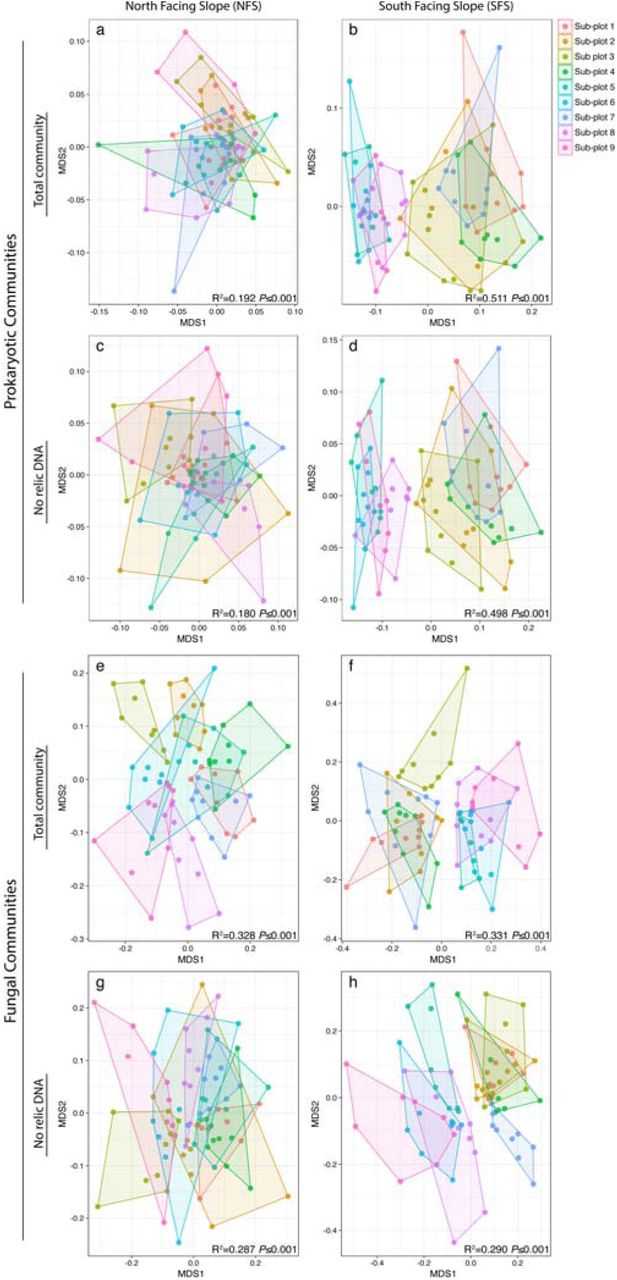
Intra-plot spatial variability in soil microbial communities persists over time on both slopes regardless of whether relic DNA is removed. NMDS plots showing the prokaryotic (a-d) or fungal (e-h) communities on the north facing slope (a,c,e,g) and south facing slope (b,d,f,h). Points are colored by sub-plot number (plot layout is illustrated in Figure 1 in the main text). Hulls connect the outermost points on each slope. PERMANOVA statistics are listed on each panel.
Removing relic DNA enhanced our ability to detect temporal changes in soil microbial communities
We investigated the temporal variability in belowground microbial communities, and the effect of relic DNA on this temporal variability, on a sub- plot basis to control for the aforementioned high degree of intra-plot spatial variability and discriminate between temporal and spatial sources of variation in microbial community structure. When limiting PERMANOVA permutations to within sub-plots over time, we found significant temporal variability for both prokaryotes and fungi in both untreated control soils (PERMANOVA R2 =0.187 P≤0.001 for prokaryotes and R2 =0.147 P≤0.001 for fungi on the NFS; and R2 =0.123 P≤0.001 for prokaryotes and R2 =0.123 P≤0.001 for fungi on the SFS) and soils that were treated to remove relic DNA (PERMANOVA R2 =0.177 P≤0.001 for prokaryotes and R2 =0.141 P≤0.001 for fungi on the NFS; and R2 =0.108 P≤0.001 for prokaryotes and R2 =0.157 P≤0.001 for fungi on the SFS). However, on average, the fungal communities on both slopes, and prokaryotic communities on the NFS were significantly more dissimilar over time after relic DNA was removed, compared to untreated control soils that contained relic DNA (Fig. 3; Kruskal-Wallis test P≤0.05). These results indicate that, while temporal signals in soil microbial communities can be identified in the presence of relic DNA, the removal of ‘legacy’ DNA from dead microbes that can persist in soil significantly enhances the ability to detect important temporal variation in the composition of soil microbial communities.

Soils without relic DNA were found to harbor microbial communities that are more dissimilar over time than in control soils containing relic DNA. (a) Prokaryotes (b) Fungi. Points are the mean community dissimilarity for a given sub-plot across all time points (n=9) for samples after relic DNA removal (no relic DNA) or untreated samples (control). Box plots illustrate interquartile range ± 1.5 × interquartile range. The horizontal line in each box plot is the median. Outliers (>1.5 × interquartile range) are shown as points outside of whiskers. Kruskal-Wallis test (K-W) P values are shown.
Temporal variability in distinct assemblages of prokaryotes and fungi are predictable from soil variables
Characterizing shifts in the relative abundances of individual microbial taxa in temporally dynamic soil systems can give important insight into the ecologies of individual taxa and, more generally, the environmental factors that influence belowground communities. Thus, we next sought to identify specific groups of taxa that exhibited correlated changes in relative abundances over time in soils after relic DNA was removed. To do this, we used local similarity analysis (LSA)23 to identify strong (local similarity score ≥0.7) and significant (q-value ≤0.001) positive pairwise microbe-microbe temporal correlations. We constructed and analyzed networks from these correlations and extracted distinct groups (modules) of microbes from NFS and SFS networks using modularity analysis24 (Fig. 4). On the NFS, the mean normalized relative abundances of 292 microbial taxa (184 bacteria and 108 fungi) were significantly correlated with at least one other taxon over time (Fig. 4a). These correlated taxa clustered into seven modules – the mean normalized relative abundances of four of these modules changed significantly with time and displayed distinct temporal trajectories (Fig. 4b). On the SFS, 291 taxa (1 archaeon, 191 bacteria and 99 fungi) were included in the network, and clustered into six modules (Fig. 4c). The relative abundances of three of these six SFS modules changed significantly with time (Fig. 4d).

Cross-domain temporal dynamics in belowground microbial communities reveals temporal niche structure. Correlation networks based on significant microbe-microbe temporal correlations for the NFS (a) and SFS (c). Nodes in (a) & (c) are individual prokaryotic or fungal taxa. Lines between nodes represent significant (q value ≤ 0.001) and strong (local similarity score ≥ 0.7) positive temporal correlations. The sizes of nodes are proportional to the number of correlations to other nodes (the degree), whereby larger nodes have more connections. Colors represent distinct modules, as determined using the modularity algorithm described in ref. 24. Boxed numbers in networks are arbitrary module numbers and match those in panels (b) and (d). Modularity analysis of each network revealed clusters of microbes that have similar temporal patterns. These temporal patterns were plotted for the NFS (b) and SFS (d). Points in (b) and (c) are the mean Van der Waerden (VdW) normalized relative abundance of all taxa in a given module. Error bars show ± SEM. The number of nodes included in each module and the PERMANOVA P value describing the relationship of the normalized relative abundances in relation to time are shown. P values marked with asterisks are significant at P≤0.001. Background is shaded by season: orange=autumn; blue=winter; green=spring; yellow=summer. See Supplementary Table 1 for taxonomic module membership.
A large proportion of the temporal variation in the mean normalized relative abundances of the modules that were found to change significantly over time could be explained by temporal variation in measured soil or environmental characteristics. At each time point, we measured a suite of soil and environmental parameters, including: snow depth, soil temperature and moisture, extractable inorganic nitrogen NO3−+ NH4−+, salinity (electrical conductivity), extractable phosphorus (P), pH, and the chromophoric properties of water-soluble organic matter (WSOM; a metric of organic matter lability25). These measured soil characteristics explained 12 to 76% of the variance in the mean normalized relative abundance of a given module (Supplementary Fig. 3). We identified two sets of modules that differed in the specific factors that predicted temporal variation. The first set of modules, containing modules 0, 3, 7 and 12, were best predicted by climactic variables, most notably soil temperature and moisture and snow depth (Supplementary Fig. 3). These results are in line with previous studies demonstrating how changes in soil temperature12, 16-18, moisture26 and snow pack14 can influence belowground microbial communities. In contrast, modules 1, 2 and 11 were best explained by changes in inorganic nutrient concentrations (nitrogen and phosphorus; Supplementary Fig. 3). While nitrogen and phosphorus inputs can have predictable27 and lasting4 effects on microbial community structure, we have a more limited understanding of how short-term seasonal variation in the availability of these nutrients can influence microbial community dynamics, despite evidence that belowground microbial communities are important mediators of soil nutrient dynamics28, 29. Our results show that a subset of soil microbes organize into modules that are responsive to these subtle changes in nitrogen and phosphorus availability. Variability in WSOM constituents did not contribute significantly to temporal variability in environmental conditions (Supplementary Fig. 4) and thus, we excluded these measures from the models describing the temporal variability of the modules. Given that previous work at these sites showed a high degree of spatial variation in WSOM distributions25, 30, we suspect that the pronounced spatial variability in WSOM distributions may have obscured our ability to detect significant effects of WSOM characteristics on the temporal dynamics of the soil microbial communities.
The construction of modules based on shared temporal patterns allowed us to identify biotic or abiotic factors that are correlated with shifts in the relative abundances of individual taxa. For example, similar to studies showing that ammonia-oxidizing archaea are particularly sensitive to changes in temperature31 and pH32, 33, we found that both temperature and pH were good predictors of the temporal distribution of module 12, which contained ammonia-oxidizing thaumarchaea (Fig. 4d and Supplementary Fig. 3). Because nitrification is often a coupled process – the oxidation of ammonium to nitrite by ammonia oxidizers, and the subsequent oxidation of nitrite to nitrate by nitrite oxidizers – we were surprised that probable nitrite-oxidizing Nitrospirae were not temporally correlated with these thaumarchaea, but were instead a part of a distinct module (module 8; Fig. 4d) that did not change significantly over time. As observed in some marine systems34, 35, we suspect that nitrification in SFS soils may be periodically uncoupled, though more work is necessary to test this hypothesis.
Our study also provides insight into the short-term temporal variation of ectomycorrhizal communities, the environmental factors that influence these patterns and other fungal and prokaryotic taxa that co-vary with ectomycorrhizal fungi. Ectomycorrhizal fungi were found on both slopes and partitioned into several modules that were significantly variable over time (modules 0, 1, 2, 3, 7, 11, and 12 in Fig. 4; Supplementary Table 1). Interestingly, some of these modules were best predicted by climactic variables (Supplementary Fig. 3; for example, those ectomycorrhizal fungi found in modules 3 and 7). Modules 3 and 7 had peak abundances in the summer months (Fig. 4), suggesting that the abundances of these ectomycorrhizal taxa were elevated during months when plant productivity peaks. However, other ectomycorrhizal fungi were found in modules best predicted by nutrient availability. These findings indicate a degree of temporal niche partitioning in ectomycorrhizal fungal communities on both slopes in response to distinct environmental conditions (Supplementary Fig. 3)
Conclusions
This study provides new evidence that the temporal dynamics of groups of prokaryotes and fungi are predictable in terrestrial ecosystems, and that a more detailed characterization of the temporal variability in soil microbial communities is critical to understanding the dynamic nature of the soil microbiome. The extensive spatial and temporal sampling design of our study allowed us to disentangle the relationships among spatial heterogeneity in microbial communities, temporal dynamics of these communities, and the effect of relic DNA on these temporal patterns. Unsurprisingly, spatial variation in community structure at both the hillslope scale, and the meter scale (intra-plot) was the dominant source of variability in this study and relic DNA had no significant effect on these patterns (Supplementary Fig. 1 and Fig. 2).
When controlling for this spatial variability, we were able to detect significant temporal shifts in microbial community composition, regardless of whether relic DNA was removed or not. We emphasize that the magnitude of the temporal variation in soil microbial communities was consistently lower than the spatial variation, even between sub-plots located only a few meters apart. This spatial variability in surface soil microbial communities was relatively stable over time, suggesting that efforts to describe spatial variation in overall community composition do not necessarily need to include samples collected across multiple time points.
We also provide new evidence that the removal of relic DNA enhances our ability to detect temporal patterns in the belowground communities. These findings support our previous hypothesis2, and predictions based on modeling21, that relic DNA can conceal temporal patterns in soil microbial communities. The presence of relic DNA, even in high amounts, does not automatically lead to relic DNA biases in other ecosystems21. However, our data do suggest that relic DNA has important effects on studies of temporal variation in soil microbial communities (and possibly in other ecosystems), and that the consequences of failing to remove relic DNA would not be apparent from single time point samples.
The belowground environment is one of the most complex and dynamic microbial habitats on Earth. By controlling for spatial and relic DNA effects on temporal variability in these soil microbial communities, we identified groups of microbes that have similar temporal dynamics and the factors that predicted their temporal distributions. A deeper understanding of relationships between soil microbiota can help resolve both the roles of individual taxa and potential ‘ecological clusters’ with emergent function. For example, taxa that covary may exhibit similar niche preferences and compete for growth substrates. In contrast, taxa belonging to a given module may broadly cue in on similar environmental signals but occupy distinct substrate niches36. Alternatively, microbes that are correlated over time may interact through cross-feeding of metabolic substrates or co-utilization of leaky functions37 - either directly or in a time-lagged manner.
Understanding the basis for shared temporal dynamics is important as microbial interactions are crucial in shaping microbial communities38 but difficult to measure directly39. Future investigations that combine cell culture, synthetic microbial communities and genomics may help resolve the specific drivers of these co-occurrence patterns36, 40.
Methods
Site description, plot design and sampling procedure
The two plots were set up on opposing slopes alongside an instrumented transect near the rain-snow transition at ∼2,530 meters elevation (approximately 40.01°N, 105.47°W), chosen on the expectation that there would be a high level of temporal variability in soil microbial communities as a result of intra-annual changes in soil moisture and temperature22. The north-facing slope (NFS) and south-facing slope (SFS) have distinct soil and vegetation characteristics and experience different water delivery patterns, particularly during snowmelt22 (Fig. 1). The NFS and SFS soils are Ustic dystrocryept (Catamount series) and Lithic haplstoll, respectively41. Soil moisture and temperature were variable over the course of the study and followed expected seasonal trends (Fig. 1). In general, the NFS had a higher soil moisture and a lower temperature than the SFS (Fig. 1). The NFS is vegetated with moderately dense Pinus contorta (Lodgepole pines) and develops a snowpack during the winter that melts in spring. In contrast, the SFS is much more sparsely vegetated with Pinus ponderosa (Ponderosa pines), intervening grasses and Arctostaphylos uva-ursi (kinnikinnick) shrubs and experiences pulses of snowmelt throughout the winter and spring. We sampled ∼10-15 random soil cores (0-5 cm, mineral soils only; 1” core diameter) within each sub-plot at each of the nine time points. The soil cores from each sub-plot were pooled, sieved to 2 mm and homogenized at each time point and partitioned for microbial community and nutrient analyses. Sample dates are reported in Supplementary Table 2. Sampling for the July 2016 sample was delayed by ∼7 days because a nearby wildfire prevented site access.
Continuous environmental measurements
Several automated measurements were collected every 10 minutes at a meteorological station located near the sample sites (see ‘Data availability’ for data source information). Each slope was instrumented with a soil temperature sensor (Campbell Scientific T-107 temperature probe), and a soil water content reflectometer (Campbell Scientific CS616) located 5 cm below ground. The daily averages from these sensors on each slope are illustrated in Fig. 1b,c. When modelling the relative mean importance of temperature and volumetric water content to module temporal distributions, we used the average of daily mean values from these sensors between sample dates, except for the first time point, which is the mean from the preceding 34 days. Snow depth was measured using digital ultrasonic snow depth sensors (Judd Communications Inc.) fitted with CR1000 dataloggers (Campbell Scientific). Snow depth is reported as mean daily snow depth between sampling points from three sensors on each slope (NFS at snow pole 3, sensors 1-3 and SFS snow pole 10, sensors 9, 11 and 15).
Discrete environmental measurements
Inorganic N pools were measured for each sub-plot at each time point except for the January 2016 sample on the NFS, sub- plots 1 and 2 and SFS sub-plot 3, where insufficient soil was collected. Sieved soils for inorganic N analyses were stored at 4°C for <72 h. Inorganic N pools were extracted from 10 g field-moist soil in 100 mL 2M potassium chloride with periodic shaking for 18 h and filtered through cellulose Whatman 1 filters. Ammonium (NH4+) was measured from these extracts on a BioTek Synergy 2 with a detection limit of 0.009 mg N L -1 and nitrate (NO3−) was measured on an OI Analytical FS-IV with a detection limit of 0.5603 μg N L- 1. Dissolved inorganic nitrogen (DIN) was calculated as the sum of NH4+ and NO3−.
Water-soluble organic matter (WSOM) was analyzed for each sub-plot at each time point except for the following plots, where insufficient sample was collected: NFS February 2016 (all sub-plots), July 2016 sub-plot 1, August 2016 sub-plots 1-7, November 2016 sub-plots 1, 2 and 5; and SFS February 2016 sub-plots 1, 8 and 9 and April 2016 sub-plot 5. Sieved soils were stored at −20°C until WSOM extraction. WSOM was extracted by leaching 10 g of soil with 50 ml 0.5 M K2SO4 following the methods described in25. The spectroscopically-active portion of the WSOM was characterized with UV-Vis and fluorescence spectroscopy. Samples were diluted to minimize the inner filter effect42 and the UV-Vis absorbance was measured from 200-800 nm in 1 nm increments using an Agilent 8453 Spectrophotometer with a 1 cm path length. Dissolved organic carbon (DOC) and total nitrogen were measured on a Shimadzu TOC-V. SUVA254, a proxy for the aromaticity of the WSOM, was calculated as the absorbance at 254 nm normalized by the DOC concentration43. Fluorescence scans were collected on a Horiba Jobin Yvon Fluoromax-4 with a 1 cm quartz cuvette and normalized to Raman units44. The fluorescence index (FI) 45 and humification index (HIX)46 were calculated from the fluorescence scans using Parallel Factor Analysis (PARAFAC) to further resolve discrete components representing different classes of fluorophores25.
Other standard soil characteristics were measured at each time point by pooling equal masses of soil from each sub-plot plot on each slope. These measurements included: pH, electrical conductivity (mmhos cm-1) and P (ppm). Standard soil chemical analyses were performed at the Colorado State University Soil Water and Plant Testing Laboratory using their standard protocols.
Relic DNA removal and DNA extraction
Relic DNA was removed as described previously2. Briefly, 0.03 g of each soil from each sub-plot pool was sub-sampled, resuspended in 3.0 mL phosphate buffered saline (PBS) (1% weight/vol slurry) and either treated with 40 µM propidium monoazide (PMA) in the dark, or left untreated as a control. Both treated and untreated samples were vortexed in the dark for 4 minutes and exposed to a 650-watt light for 4 × 30 s light:30 s dark cycles to activate PMA in treated samples. Light-exposed samples were frozen at −20°C until DNA extraction. DNA was extracted from 800 µL of PMA treated and untreated soil slurries using a PowerSoil-htp 96 well soil DNA Isolation kit (MoBio) following the manufacturer’s instructions, except 770 µL was used in the C2 step. All samples and 27 ‘no soil’ negative controls were randomized into these 96 well DNA extraction plates and extracted simultaneously.
Amplicon sequencing and analytical methods
For sequence-based analyses of 16S rRNA and ITS marker regions, we used the approaches described previously2. Briefly, we amplified each sample in duplicate in 25 μl PCR reactions containing: 12.5 μl of Promega GoTaq Hot Start Colorless Master Mix; 0.5 μl of each barcoded primer (bacterial 16S: 515F 5′-GTGCCAGCMGCCGCGGTAA-3′ & 806R 5′-GGACTACHVGGGTWTCTAAT-3’; fungal ITS: 5′-CTTGGTCATTTAGAGGAAGTAA-3′ & ITS2 5′-GCTGCGTTCTTCATCGATGC-3′); 10.5 μl water; 1 μl of template DNA. Program: 94°C for 5 min, followed by 35 cycles of (94°C 45 s; 50°C 60 s; 72°C 90 s) and a final extension 72°C 10 min. Duplicate PCR reactions for each sample were pooled, cleaned and normalized using the ThermoFisher Scientific SequalPrep Normalization Plate kit. Cleaned and normalized amplicons were pooled, spiked with 15% phiX and sequenced on an Illumina MiSeq using v2 500-cycle paired end kits. The samples were sequenced in four batches total – two for prokaryotes and two for fungi. The first two sequencing runs (one each for prokaryotes and fungi) contained all treatments and control samples up to and including the May 2016 samples. The last two sequencing runs (one each for prokaryotes and fungi) two contained samples collected on July 2016 and thereafter, plus control samples. We analyzed the ‘no soil’ controls to determine whether there were potential sequencing batch effects across the runs for prokaryotes or for fungi that could be detected in the community composition of these controls. We found no significant difference in the ‘no soil’ controls for prokaryotes (rarified to 89 reads to include all controls; PERMANOVA R2=0.028; P=0.677) or fungi (not rarified to include all controls; PERMANOVA R2=0.028 P=0.613) that would be indicative of batch effects. Reads were processed as described in (ref. 27). Briefly, raw amplicon sequences were demultiplexed according to the raw barcodes and processed with the UPARSE pipeline47. A database of ≥97% similar sequence clusters was constructed in USEARCH (Version 8)48 by merging paired end reads, using a “maxee” value of 0.5 when quality filtering sequences, dereplicating identical sequences, removing singleton sequences, clustering sequences after singleton removal, and filtering out cluster representative sequences that were not ≥75% similar to any sequence in Greengenes (for prokaryotes; Version 13_8)49 or UNITE (for fungi)50 databases. Demultiplexed sequences were mapped against the de novo constructed databases to generate counts of sequences matching clusters (i.e. taxa) for each sample. Taxonomy was assigned to each taxon using the RDP classifier with a threshold of 0.551 and trained on the Greengenes or UNITE databases. To normalize the sequencing depth across samples, samples were rarefied to 10,159 and 5,000 sequences per sample for the 16S rRNA and ITS analyses, respectively. Functional predictions for fungal taxa were obtained using FUNGuild52.
Statistical analyses
Calculations of community dissimilarity and all other analyses were conducted on a reduced dataset because of the spatial and temporal heterogeneity. That is, we wanted to understand the temporal variation of microbes that are consistently present across the sub-plots and over time. When comparing slope differences, we included only taxa that were present on at least one slope i) with a mean read abundance of greater than 81 or 40 reads after rarefaction, for prokaryotes and fungi, respectively across all samples (an average of one (prokaryotes) or 0.5 (fungi) reads per sub-plot, per time point); and were ii) present in more than 27 samples (1/3 of all samples). Second, we investigated only those taxa that were, on average, ≥ 0.1% of the community across all samples. When investigating within-plot differences, we focused on only the taxa within that plot that met the above parameters. We emphasize that these filtering steps were deliberately stringent to enable robust temporal analyses of taxa that are consistently present both spatially and temporally. Bray-Curtis distances were calculated on this subset using the mctoolsr R package. Bray–Curtis dissimilarities were calculated on square root transformed taxon relative abundances.
Temporal analyses and network construction
We identified significant temporal correlations in the relative abundances of individual taxa derived from soils that were treated to remove relic DNA using extended Local Similarity Analysis (eLSA)23 with the following parameters: lsa_compute -s 9 -r 9 -p perm. We defined significant temporal associations as those with a local similarity (LS) score ≥0.7 (i.e.-strong to very strong correlations) and a q value ≤ 0.001. Pairs of significantly correlated taxa were analyzed in Gephi (version 0.8.2). Network modularity was calculated by implementing the ‘modularity’ function24 built in within Gephi, with a resolution setting of 1.0 for both slopes. Node IDs (individual taxa) belonging to the same module were extracted to delineate temporal patterns. Normalized relative abundances for each node ID were calculated using the tRank command in the multic R package.
Random forest analysis
For each slope, we used Random Forest53 modeling to first identify those measured environmental and soil variables that were significant (P ≤ 0.05) predictors of time, using time as a response variable (Supplementary Fig. 4). These significant environmental factors are expected to predict changes in module abundance over time (Supplementary Fig. 3). We then conducted a second round of Random Forests analysis with the significant environmental predictors to identify the most important environmental factors or soil characteristics that predicted the mean normalized relative abundances of each module (see ref. 54 for a similar approach). The importance (increase in mean square error %) and significance of each predictor was computed for each tree and averaged over the forest (9999 trees) using the rfPermute R package. Significant predictors were defined as those with a P value ≤ 0.05. Samples for which environmental and soil characteristics were missing because of insufficient sample were excluded from random forest and spearman correlation analysis.
Data Availability
Raw DNA sequence data, the corresponding mapfile and all soil and environmental characteristics are available on figshare.com: 10.6084/m9.figshare.6710087. Snow depth data are available through the Boulder Creek Critical Zone Observatory website: http://criticalzone.org/boulder/data/dataset/2423/. Temperature data for the NFS and SFS are available through the Boulder Creek Critical Zone Observatory website http://criticalzone.org/boulder/data/dataset/2426/.
Acknowledgements
We thank Gordon Bowman, Youchao Chen, Matt Gebert, Rebecca Gross, Evan Lih, Emily Morgan, Dillon Ragar, Nathan Rock and Joel Singley for assistance setting up plots, sampling and nutrient analyses. We also thank David Needham for assistance with LSA and Albert Barberán for critical feedback on the manuscript. Funding to support this work was provided by grants from the National Science Foundation EAR 1331828, EAR 1461281, and DEB 1556753 to N.F., and a Visiting Postdoctoral Fellowship award to P.C. from the Cooperative Institute for Research in Environmental Sciences at the University of Colorado.
References


