

Abstract
Psychophysiological interaction (PPI) and beta series correlations (BSC) are two commonly used methods for studying task modulated connectivity on functional MRI (fMRI) data. So far there are no comprehensive tutorials to explain these two methods, and the relationships between these two have not been established. In the current paper, we explained in detail what the two methods measure, and how these two methods are related. We elucidated why the PPI approach always measures connectivity differences between conditions. This is in contrast with the BSC approach, which can measure the absolute connectivity in a specific task condition. By explaining the deconvolution process of the observed blood-oxygen-level dependent (BOLD) signals from fMRI with hemodynamic response function, we explicated that PPI can measure the differences of correlations of trial-by-trial variability in different conditions. Therefore, when comparing connectivity between different conditions, PPI and BSC methods could in principle generate similar results. In addition, we established that when modeling multiple conditions in PPI analysis, PPI models calculated from direct contrast between conditions could generate identical results as contrasting separate PPI terms coding each of the conditions (a.k.a. “generalized” PPI) if the models were defined correctly. We also reported empirical PPI and BSC analyses on fMRI data of a stop signal task to support our points.
1. Introduction
Although the majority of fMRI studies are task-based, because of its simplicity, resting-state fMRI has emerged as an alternative method to measure functional connectivity (Biswal et al., 1995, 2010). The entire scan period of resting-state can be treated as a single state. Therefore, correlation coefficients of time series between different brain regions could be used to study functional connectivity (Biswal et al., 1995). For task based fMRI, there are typically multiple task conditions within a scan. The challenge is to estimate functional connectivity differences between different conditions. There are primarily two methods that have been developed to study functional connectivity differences for task fMRI data, namely psychophysiological interaction (PPI) (Friston et al., 1997) and beta series correlation (BSC) (Rissman et al., 2004). There is also dynamic causal modeling (DCM) that can be used for this purpose (Friston et al., 2003). However, this method is restricted to a small number of regions of interest, and is largely hypothesis-driven. Therefore, we did not cover DCM in the current paper.
PPI was first proposed by Friston and colleagues based on the interaction term between a physiological variable of a regional time series and a psychological variable of task design in a regression model (Friston et al., 1997). Thereafter, a major update was made to perform deconvolution on the time series from the seed region, so that the interaction term could be calculated at the “neuronal level” rather than at the hemodynamic response level from fMRI signals (Gitelman et al., 2003). Later, McLaren and colleagues proposed a “generalized PPI” approach for modeling PPI effects for more than two conditions (McLaren et al., 2012). They proposed to model each task condition with reference to all other conditions and then compared the PPI effects between the conditions of interest, rather than directly calculating PPI effects between the two conditions. Recently, we found that the interaction between not centering the psychological variable and imperfect deconvolution process may lead to spurious PPI effects (Di et al., 2017), and the deconvolution may be not a necessary step for PPI analysis on block-design data (Di and Biswal, 2017).
The BSC method, on the other hand, was primarily proposed for event-related designs (Rissman et al., 2004). By modeling the activations of every trial separately in a general linear model (GLM), one can estimate a series of beta maps for the series of trials. Therefore, connectivity in different task conditions can be calculated and compared by correlations of trial-by-trial beta series variability in different conditions. The relationships between the BSC and PPI have not yet been clearly explained. Nevertheless, one study has suggested that BSC method is more suitable for event-related data than PPI (Cisler et al., 2014). However, our recent study using a large sample did not support this conclusion (Di and Biswal, 2018).
In the current paper, we have provided an in depth explanation of the PPI and BSC methods, and explain the relationships and differences between these two methods. In order to do so, we need to first clarify why the PPI method always measure connectivity differences between conditions. In addition, we explained the deconvolution process implemented in the calculation of PPI term, which will help to understand how PPI can measure the differences between the trial-by-trial correlation in one condition and the moment-to-moment correlation in the remaining time points. Because of this, the PPI differences between conditions and the BSC differences between conditions can in principle measure the same task modulated connectivity. We have used both simulations and real fMRI data of an event-related designed stop signal task to illustrate our points.
1.1. Modeling of task main effects
We start with the modeling of the main effects of task conditions. Assuming a simple task design of two conditions A and B, in a regression model, we can use two regressors to represent the two conditions in two different ways. First, we can use the two regressors to represent the specific effect of each condition, i.e. using 1 to represent the modeled condition and 0 for the other condition (Figure 1A). However, a constant term that represents the overall effect is usually added in a regression model, which is also known as the intercept. Therefore, we only need to add one more regressor to represent the differential effect between the two conditions (Figure 1B). The two models are mathematically equivalent, because the two regressors in model 1A could be expressed as linear combinations of the two regressors in model 1B, and vice versa. However, because of the differences model strategies, the meanings of the same regressor from the two models (the first regressor from model 1A and the second regressor from model 1B) have changed. In model 1A, the regressors represent the condition specific effects. In model 1B, however, the second regressor actually represents the differential effect of conditions A and B. This is important regarding the interpretation of the estimated effects of these regressors. Mathematically, model 1B can be expressed as:
 where XPsych represents the differential effects between conditions A and B, i.e. the psychological variable. y represents the brain signal in a brain region or voxel. β0 and β1 are parameter estimates that represent the mean effect and differential effect of the two conditions, respectively.
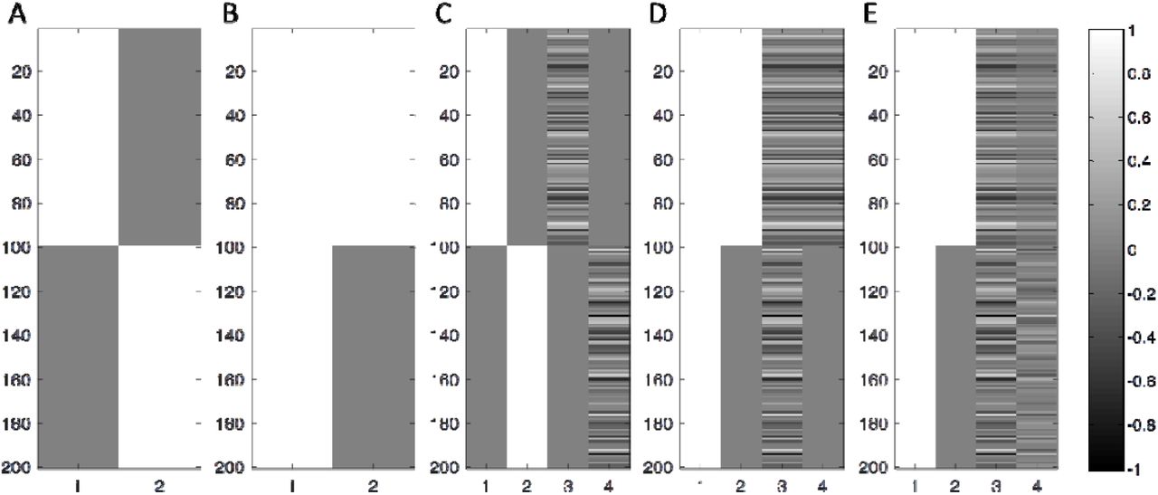
Main effects and interaction models for two experimental conditions. The main effects of two conditions can be modeled as two separate regressors (A), or modeled as the differential and mean effects of the two conditions (B). When modeling the interaction terms of the experimental condition with a continuous variable, the same two strategies could be used as C and D. E illustrates how the interaction term was changed (from D) when centering the psychological variable before calculating the interaction term. Because of the different modeling strategies, the interpretations of the regressors changed.
Another important point from equation 1 is that although XPsych is usually represented as 1 and 0 for the two conditions, the constant component in the xpsych can be explained by the constant term in equation 1 (see supplementary materials). Thus, whether centering the XPsych variable will not affect the effect estimate of β1, neither the interpretation of β1. β1 always represents the differential effect of the two conditions.
1.2. Functional connectivity and connectivity-task interactions
The term functional connectivity was first defined by Friston (Friston, 1994) as temporal correlations between spatially remote brain regions. Assuming that the functional connectivity is the same during the period of scan, e.g. in resting-state, it is straightforward to calculate correlation coefficients between two brain regions to represent functional connectivity. In a more general regression form, the model can be expressed as:
 where XPhysio represents the time series of a seed region. β1 in this case represents the correlation between seed and tested voxel, i.e. functional connectivity.
In most of task fMRI experiments, researchers design different task conditions within a scan run, so that the effect of interest becomes the differences of temporal correlations between the conditions. We can combine equations 1 and 2 to include both the time series of a seed region (the physiological variable) and the psychological variable representing task designs into a regression model. Most importantly, the interaction term between the psychological and physiological variables can also be included. For the simplest scenario with only one psychological variable (two conditions), the psycho-physiological interaction (PPI) model can be expressed as:

Equation 3 can be illustrated figuratively in Figure 1D. Combine the two terms with XPhysio, equation 3 can be expressed as:

Equation 4 shows that the relationship between the seed region XPhysio and test region y is: β2+β3 XPsych, which is a linear function of XPsych. Therefore, a significant β3 represent significant task modulations on connectivity.
Like the interpretation of task main effects, the interpretation of the PPI effect depends not only on the coding of the psychological variable, but also the inclusion of other variables in the model. In equation 3 the main effect of time series XPhysio is included. We can think about the time series main effect XPhysio and interaction effect XPhysio · XPsych as the second order counterparts of the constant effect and main effect of XPsych in equation 1. Here the point is that adding this time series main effect affects the interpretation of the interaction term. Because the overall relationship with the seed time series has been modeled, the interaction term measures the differences of the relationships between the two conditions. We note that if XPhysio main effect was not added, the interaction term could actually be calculated with each condition separately (Figure 1C). Then the third and fourth columns in Figure 1C can represent condition specific connectivity effects. Here again the same interaction terms from the two models (regressor 3 in model 1C and regressor 4 in model 1D) represent different effects.
In addition, because the main effects of XPhysio and XPsych are both added in the interaction model (equation 3), the interpretation of the interaction term should refer to the demeaned version of the two variables. Because the XPsych is usually coded as 0 and 1 for the two conditions, the demeaned version of XPsych will be −0.5 and 0.5 instead. This will make the interaction term look very different (column 4 in Figure 1E compared with that in Figure 1D). However, the estimated interaction effect will be identical, because the difference between the two interaction terms is the physiological main effect, which has been taken into account in the model (For real fMRI data, however, the centering matters because the main physiological main effect interacts with the deconvolution process to produce spurious PPI effects (see Di et al., 2017 for more details)).
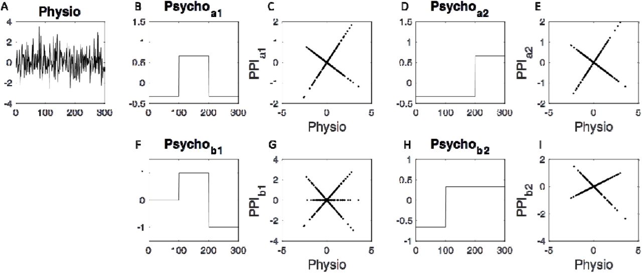
To better illustrate the meaning of PPI effect, we plot the PPI effect against the original time series XPhysio. PPI can be represented as a projection of the seed time series, so that the PPI represents different relationships with the seed region in different task conditions. When the psychological variable is coded as 1 and 0 for the two conditions, the PPI represents a perfect relationship with the seed time series in the “1” condition and a smaller effect in the “0” condition, which is reflected as a horizontal line in Figure 2D. When the mean of the psychological variable is removed before calculating the interaction term, the projection rotates clockwise compared with the non-centered version (Figure 2G). However, what is reflected in the two projections are the same, which is the difference between the two conditions. In real cases, there may be positive connectivity in condition A and no connectivity in condition B, or there may be no connectivity in condition A but negative connectivity in condition B. In both cases, PPI can capture the differential connectivity effects. This logic is similar to the main psychological effect explained in section 1.1, which reflects the differences between the two conditions but not the effect in one condition.

The interaction term as a projection of the continuous (physiological) variable. A continuous variable (A) is multiplied with a psychological variable (B or E) to form an interaction term (C or F), which can be plotted against the continuous variable itself (D or G). When the psychological variable is modeled as 0 and 1 (B), the projection will result in a horizontal line (y = 0) during the 0 period and a y = x line during the 1 period. But usually the psychological variable is centered (D). Therefore, the projection represents y = −0.5 x and y = 0.5 x lines during the two conditions, respectively.
1.3. More than two conditions
When the number of conditions increases, more regressors are needed to represent each condition, with typically n regressors for n conditions. Because there is always a constant term, or intercept, in the regression model, we actually need n – 1 additional regressors. This is convenient for most task fMRI studies, because there is usually an implicit baseline conditions in an fMRI experiment. For event-related design, it is even difficult to define the implicit baseline condition. Therefore, we can include all other experimental conditions, and leave the baseline condition out of the model. Because of the inclusion of the constant term, we should always keep in mind that the regressors included in the model represent differences of between the modeled condition with respect to all the other conditions, rather than the specific effect of a condition.
Let us assume a task design with task conditions A and B together with a baseline condition R. In this case, the effect of interest is the differences between conditions A and B. A natural way to model the three conditions is to use two regressors to represent A and B, separately (Figure 3B and 3D). We could then calculate the interaction terms of the two psychological regressors separately with the seed time series. The two interaction terms represent the correlation differences between A − (B + R) and B − (A + R), respectively. A contrast of [A − (B + R)] – [B − (A + R)] = 2 × (A − B) can then be used to examine the differential effect between A and B. This strategy is usually referred to as “generalized PPI” (McLaren et al., 2012). One can also directly contrast A with B to define a new psychological variable.
Illustrations of “generalized” PPI and contrast PPI for three conditions. Because of the inclusion of the constant term, two psychological variables are needed to model the differences among the three conditions. In the “generalized” PPI approach, the two psychological variables are demonstrated as B and D, which represent one specific condition against the other two conditions. The corresponding PPI terms were plotted against the physiological variable (A) in C and E. In the contrast PPI approach, the two psychological variables are demonstrated as F and H, which represent the differential and mean effects of the last two conditions. The corresponding PPI terms were plotted against the physiological variable (A) in G and I.
It can be achieved in SPM by defining contrast value 1 to condition A, and −1 to condition B. However, one should not forget that there is the third condition R, which will be implicitly left as 0. Simply doing this is problematic, because it assumes that the relationship in the R condition is somehow between what is in A and B conditions (Figure 3G). Because there are three conditions per se, we have to use two variables to model the differential effects among the three conditions. In this case, we could include one more psychological variable to represent the differential effect between the mean effect of A and B and the effect of R (Figure 3H). The interaction term of this psychological variable with the seed time series can effectively remove the differential effects of relationships between conditions A/B and condition R (Figure 3I). Therefore, if we include the PPI terms of 3H and 3I in the model, the effect of 3G will be equivalent to the differential effects of 3C and 3E. In the original paper of McLaren, it has been shown that the “generalized PPI” approach performed better than the contrast PPI. It is probably because of the neglect of the R condition. However, if the psychological variables are modeled correctly, the two methods should provide the same results.
1.4. Block design and event-related design
So far we have divided the observations of different task conditions into different groups regardless of the orders of the observations. For fMRI, the task conditions need to be designed carefully to accommodate the properties of hemodynamic responses following the neural activity changes due to the task designs. There are usually two types of designs, i.e. block design and event-related design. For block design, a task condition is broken into separate short blocks, and the blocks are repeated for several times within a scan run. For event-related design, each trial is a unit to evoke hemodynamic responses. The temporal distance between trials should be designed carefully, so that the hemodynamic response for each trial could be effectively separated. The psychological variable for event-related design is modeled as a series of impulse function at the onset of the trials with remaining time points as 0. The mathematical meanings of the psychological variables in a block design and an event-related design are the same, which represent the differences between conditions. And it is the same for the PPI effects as well. For the block design, we can think of PPI as a measure of the differences of moment-to-moment correlations between conditions. The event-related design can be thought of as the correlation of activations at each trial onset time point compared with the correlation of all remaining time points. In other words, it measures the correlations of trial-by-trial activation variability in one condition compared with the correlations of moment-to-moment activations in the remaining time points. Again, it measures the differences of correlations between the two conditions but not the correlation of the trial condition itself.
1.5 Convolution and deconvolution
One important aspect of fMRI is the asynchrony between the (hypothetical) neuronal activity and the observed blood-oxygen-level dependent signals (BOLD). Imagine that a single trial elicits neural activity that is typically treated as an impulse function with short event duration. This event or short neural activity gives rise to a delayed hemodynamic response, usually called hemodynamic response function (HRF) (Figure 4A). If we have a study design or hypothetical neural activity, the expected BOLD signal can be calculated as a convolution of the neural activity time series with the HRF. Because the fMRI data are discrete signals, the convolution can be converted into a multiplication of the neuronal signal with a convolution matrix defined according to the HRF. If we use z to represent variables at the neuronal level, and x to represent variables at the BOLD level, the convolution can be expressed as:
 where * represents the convolution process, and o represents matrix multiplication, h is the HRF, and H represents the matrix form of h. Each column of H represents a HRF with a different start point (Figure 4B). Therefore, the multiplication of a neural time series H with z can be represented as a summation of the hemodynamic responses of z at every time point.

Hemodynamic response function h(A) and its corresponding convolution matrix H(B).
In fMRI data analysis, we typically hypothesize that an experimental manipulation will evoke immediate neural response (relative to the time scale of BOLD responses). The expected BOLD responses to the experimental manipulations could then be represented as the convolution of the psychological variable ZPsych (a box-car function or a series of impulse functions) with the HRF. Thus, the BOLD level prediction variable XPsych can be calculated from ZPsych as the following:

On the other hand, we have a time series of a region XPhysio, which is already at the BOLD level. Therefore, we can directly calculate the interaction term by multiplying XPhysio with XPsych.

This is how PPI was calculated when the method was originally proposed (Friston et al., 1997). The limitation of this approach is that it calculates the interaction at the BOLD level, but the real interaction would happen at the hypothetical “neuronal” level.
Given the BOLD level time series x, we can perform the inverse process of convolution, i.e. deconvolution to recover the time series z at the neuronal level from equation 5. However, the H matrix is a square matrix, and deconvolution cannot be simply solved by inversing the H matrix. In addition, in real deconvolution problem like the fMRI signals, there are always noises in the recorded signals that need to be taken into account. Therefore, the deconvolution problem has to solve the following model with a noise component ε.

Because H cannot be directly inversed, some computational methods like regularization are needed to reliably obtain z. In SPM, it additionally substitutes z with Discrete Cosine Series, so that the estimation of temporal time series was transformed into frequency domain (Gitelman et al., 2003). And the regularization is applied to specific frequency components.
Using deconvolution, a seed time series XPhysio could be deconvolved to the neuronal level time series ZPhysio and multiplied with the neuronal level psychological variable. The interaction term could be convolved back into BOLD level.

Comparing X1PPI and X2PPI, we know that they are not mathematically equivalent. The later one is more appropriate to describe neural interactions. However, empirically, the PPI terms calculated with the two ways could be very similar for block designs (Di and Biswal, 2017). On the other hand, deconvolution is an ill-posed problem, and relies on sophisticated computational techniques, which may not work well in some circumstances. Therefore, it has been suggested that at least for block design, deconvolution may not be necessary (Di and Biswal, 2017; O’Reilly et al., 2012). The deconvolution approach may still be important and necessary for event-related design.
1.6. Beta series correlations
BSC is based on a simple idea of calculating correlations of trial-by-trial variability of activations. Therefore, instead of modeling different task conditions, BSC models every trial’s activationss to obtain a beta map for each trial. For each trial, an impulse function at the trial onset is defined and is convolved with HRF. Therefore, in a GLM model for BSC analysis there is the same number of regressors as the number of trials plus a constant term. The model can be expressed as the following:
 where n represents the number of trials, and Xn represents the modeled response of the trial n. The model can be expressed in a matrix form:
 where β represents a vector of βS that represent the activations of different trials (plus a β0 for the constant term). The matrix X is the design matrix (see Figure 5 for examples). One can then calculate cross-trial correlations of the beta values between regions to represent functional connectivity. Since there are usually more than one experimental condition, the beta series can be retrospectively grouped into different conditions, and the beta series correlations can be compared between the conditions.

Example design matrices for beta series correlation (BSC) analysis for a slow event-related design (Flanker task) (A) and a fast event-related design (Stop signal task) (B). Each regressor (column) other than the last one represents the activation of a trial, while the last column represents the constant term. The sampling time is 2 s for both of the two designs. The intertrial intervals for both the designs were randomized to optimize the estimations of hemodynamic responses. The mean intertrial intervals are 12 s for the Flanker task and 2.5 s for the Stop signal task, which result in 24 trials and 126 trials, respectively.
The hemodynamic response typically reaches the peak at 6 s after the trial onset and returns back to the baseline after about 15 s. To avoid overlaps of hemodynamic responses between trials, conventional event-related experiments use slow designs with intertrial interval usually greater than 10 s. Figure 5A demonstrates a beta series GLM for a slow event related design from a Flanker task (Kelly et al., 2008). Considering the sampling time of 2 s for typical fMRI, the design matrix of Figure 5A can be reliably inversed (24 trial regressors vs. 146 time points). However, fast event-related design is becoming popular, because of its efficiency of maximizing experimental contrasts. The intertrial interval could be close to the sampling time of fMRI for some designs. Figure 5B demonstrated a beta series GLM for a fast event-related design from a stop signal task (Di and Biswal, 2018). In this case the mean intertrial interval is 2.5 s. It can be seen from Figure 5B that the number of regressors becomes closer to the number of time points (126 trial regressors vs. 182 time points). This matrix cannot be reliably inversed using ordinary least squares (OLS) method, and some sophisticated computational methods may be helpful to resolve the problem, e.g. using regularization or modeling a single trial against all other trials to reduce the number of regressors (Mumford et al., 2012).
The beta values in the beta series model typically represent BOLD level activations at each trial. However, in an extreme case when the trials are presented at every time point, the beta series GLM model will become exactly the same as the convolution matrix in Figure 4B. This suggests a link between the beta series model and deconvolution. For the deconvolution model, the response for every time point was modeled (equation 8). For the beta series GLM model, however, only the time points of trial onsets were modeled (equation 11). Nevertheless, the goals of the two models are the same to measure activity at the modeled trial onsets. Here the activations at the neuronal level at the trial onset are equivalent to the activations at the BOLD level of the trials. Therefore, we can think of beta series modeling as a modified deconvolution process, even though strictly speaking it is not. Given this, we can discuss the relationships between the PPI and BSC methods.
1.7. The relationship between PPI and BSC
As described in previous sections, the BSC method selectively picks the time points at trial onsets, and computes trial-by-trial correlations between brain regions. The PPI, on the other hand, always measures connectivity differences as coded by a psychological variable. Therefore, an absolute beta series correlation in one condition is not directly comparable to a PPI effect. However, what are usually of interest are the connectivity differences between conditions. In this case, we can compare beta series correlation differences between conditions. Considering the same task design with experimental conditions A, B, and a baseline R, we can directly compare the beta series correlations between conditions A and B (i.e., A − B). If PPI was modeled using the “generalized” approach, we can have the two PPI effects representing A − (B + R) and B − (A + R). These two PPI effects can be directly contrasted, which result in the contrast of 2 × (A − B). Therefore, in theory the BSC and PPI methods measure the same connectivity differences.
Although theoretically PPI and BSC could measure the same task modulated connectivity, the results of PPI and BSC on real fMRI data may not be identical. Several factors may contribute to the differences. The first is the different approaches to deconvolution. The deconvolution method implemented in SPM uses Discrete Cosine Series to convert the temporal domain signal into frequency domain, and then applies regularization on the frequency domain to suppress high frequency components in the signals. For BSC method, if it is a slow event-related design, the design matrix includes all the trials to obtain all the trial activations at the same time. For a fast event-related design, some regularization methods may be used to obtain the beta series, or the model should be modified to contain one regressor of one trial and one regressor of all other trials to reduce the number of regressors (Mumford et al., 2012). The efficiency and reliability of these mentioned methods are difficult to determine and compare. And it may depend on the intertribal intervals of a design (Abdulrahman and Henson, 2016; Mumford et al., 2014; Visser et al., 2016), or different brain regions due to different amount of HRF variability (Handwerker et al., 2004). Therefore it is difficult to make a definite conclusion at the current point about which method is better over the other.
Another difference may be the differences in measure of connectivity. By using a regression model PPI essentially measures covariance differences between conditions. On the other hand, BSC typically uses correlation coefficients. It is still largely unknown how the variability of BOLD signals changes in different task conditions. But the differences in measures of covariance and correlations can certainly give different results. For BSC, one can choose different measures of connectivity, e.g. Pearson product-moment correlation, Spearman rank correlation, covariance, or even use the similar beta series by task interaction to estimate connectivity differences. However, it is still an open question about which method is optimal for the purpose of connectivity estimation.
1.8. An empirical demonstration
To summarize, we have explained the meanings of PPI and BSC analyses, as well as the relationships between them. PPI always measures connectivity differences as coded by the psychological variable, while BSC could measure connectivity in specific condition. When comparing connectivity between conditions, PPI and BSC methods should in principle generate similar results, although different ways to handle deconvolution and different measures of connectivity may contribute to the differences in results. For PPI analysis, there may be multiple ways to model task conditions in PPI analysis. But if done correctly, different approaches in principle should generate the same results.
In the following sections, we describe PPI and BSC analyses on a fast event-related designed stop signal task. In this task there were two experimental conditions (Go and Stop) in addition to an implicit baseline. The connectivity differences between the Stop and Go conditions have been reported in our previous work (Di and Biswal, 2018). To better illustrate the relationships between PPI and BSC methods, we reported connectivity measures of PPI and BSC methods for simple conditions and condition differences. In addition, we will compare different measures of BSC, i.e. Pearson’s correlation, Spearman’s correlation, and covariance, and examine whether these measures will affect BSC results. Lastly, we will compare PPI results using the “generalized PPI” approach with direct contrast approach where the differential and mean effects of the two conditions are both modeled. We will show that these two modeling approaches can provide identical connectivity difference measures.
2. Materials and methods
2.1. Dataset and designs
In a previous study, we have reported PPI and BSC results of connectivity differences between the Stop and Go conditions (Di and Biswal, 2018). In the current manuscript, we have used the same data to illustrate how different PPI models could give rise to the same results and how the PPI and BSC methods can be similar or different. This dataset was obtained from the OpenfMRI database, with accession number ds000030. Only healthy subjects’ data were included in the current analysis. After removing subjects due to large head motion, a total of 114 subjects were included in the current analysis (52 females). The mean age of the subjects was 31.1 years (range from 21 to 50 years). In the stop signal task, the subjects have to indicate the direction (left or right) of an arrow presented in the center of the screen. For one fourth of the trials, a 500 Hz tone was played shortly after the arrow, which signaled the subjects to withdraw their response. In a single fMRI run, there were 128 trials in total in total, with 96 Go trials and 32 Stop trials. The task used a fast event-related design, with a mean intertrial interval of 2.5 s (range from 2 s to 5.5 s). For a subset of 103 subjects, we also analyzed their resting-state fMRI data. The exclusion of subjects were due to large head motions in either the resting-state run or other task runs that were not included in this paper.
The fMRI data were collected using a T2*-weighted echoplanar imaging (EPI) sequence with the following parameters: TR = 2000 ms, TE = 30 ms, FA = 90 deg, matrix 64 × 64, FOV = 192 mm; slice thickness = 4 mm, slice number = 34. 184 fMRI images were acquired for each subject for the stop signal task, and 152 images were acquired for the resting-state run. The T1 weighted structural images were collected using the following parameters: TR = 1900 ms, TE = 2.26 ms, FOV = 250 mm, matrix = 256 × 256, sagittal plane, slice thickness = 1 mm, slice number = 176. More information about the data can be found in (Poldrack et al., 2016).
2.2. FMRI preprocessing
The fMRI image processing and analysis were performed using SPM12 (v6685) (http://www.fil.ion.ucl.ac.uk/spm/) and MATLAB codes in MATLAB R2013b environment (https://www.mathworks.com/). The anatomical image for each subject was first segmented, and normalized to standard MNI (Montreal Neurological Institute) space. The first two functional images were discarded, and the remaining images were realigned to the first image, and coregistered to the subject’s own anatomical image. The functional images were then transformed into MNI space by using the deformation images derived from the segmentation step, and were spatially smoothed using a 8 mm FWHM (full width at half maximum) Gaussian kernel.
2.3. PPI analysis
The first step of PPI analysis is to build a GLM model of task regressor, which can also be used to obtain task related activations. In the current analysis, the Go and Stop conditions were modeled separately as series of events. In SPM, the durations of the events are usually set as 0 to reflect the impulse nature of the events. But for PPI analysis, the problem is that after deconvolution, the time series were up-sampled (16 times by default). If the duration was set as 0, then the neuronal level psychological variable only has a time bin of TR/16 of one, leaving all other time bins as 0. This may be problematic when multiplying this psychological variable with the deconvolved seed time series. Considering that the calculated PPI term will be convolved back with HRF, which resembles a low pass filtering, the effects of trial duration may not be that significant. In the previous analysis, we set the duration to 1.5 s, which is the actual duration of the trial. We have also shown in the supplementary materials that setting the event duration as 0 produce very similar results as those with 1.5 s duration. In addition to the two task variables, 24 head motion regressors and one constant regressor were also included in the GLM model. After model estimation, the times series from 164 ROIs were extracted. The head motion, constant, and low frequency drift effects were adjusted during the ROI time series extraction. These 164 ROIs were adopted from previous studies (Di and Biswal, 2018; Dosenbach et al., 2010) to represent whole brain coverage. The following connectivity analyses using PPI and BSC were all performed on the ROI basis.
The PPI terms were calculated using the two different approaches, i.e. “generalized” PPI and contrast PPI. In the first approach, we first used the contrasts [1 0] and [0 1] to define two psychological variables to represent the Go and Stop conditions, separately. The PPI terms were then calculated accordingly using the deconvolution method. The calculated PPI terms were combined together with the original model to form a new GLM model for PPI analysis:

This model included one constant term, two regressros of task activations of the Go and Stop condition, one regressor of the time series of a seed region, and two regressors of PPIs. Because the dependent variable y is also a ROI time series, where the head motion effects have already been removed, the head motion regressors were no longer included in the PPI models. After model estimation, we calculated β5 – β4 as the connectivity effects between the Stop and Go conditions.
We also applied the second model where the differential and mean effects of the Stop and Go conditions were modeled. The differential effect was defined using the contrast [-1 1], and the mean effect was defined using the contrast [1/2 1/2]. The GLM for the contrast PPI analysis was as follow:

The β5 could be used for group level analysis to present connectivity differences between the Stop and Go conditions.
For each subject, the PPI models were built for each ROI, and were fitted to all other ROIs. The beta estimates of interest or contrast of interest were calculated between each pair of ROI, which yielded a 164 by 164 matrix for each effect. The matrices were transposed and averaged with the original matrices, which yielded symmetrical matrices. One sample t test was performed on each element of the matrix for an effect of interest. False discovery rate (FDR) correction was used at p < 0.05 to identify statistical significant effects in a total of 13,366 effects (164 × (164 − 1)/2).
2.4. Beta series analysis
As has been shown in our previous paper (Di and Biswal, 2018), modeling all trials together in a single model could not work for the beta series analysis. Therefore, we only reported the results from the single-trial-versus-other-trials method (Mumford et al., 2012). We first built a GLM model for each trial, where the first regressor represented the activation of the specific trial and the second regressor represented the activations of all the remaining trials. The 24 head motion parameters were also included in the GLMs as covariance. The duration of events was set as 0. After model estimation, beta values of each ROI were extracted for each trial. The beta series of each ROI were sorted into the two conditions, and connectivity measures across the 164 ROIs were calculated. In our previous work, we used Spearman’s rank coefficients to avoid the assumption of Gaussian distribution of beta values or spurious correlations due to outliers. In the current analysis, we also calculated Pearson’s correlation coefficients and covariance to examine whether these two measures may give more reliable estimates of connectivity. Before calculating the covariance, the whole beta series (Go and Stop together) of a ROI were z transformed. All of the three measures yielded a symmetrical matrix for each subject. The correlation matrices (either Pearson’s or Spearman’s) were transformed into Fisher’s z matrices. For a single condition, the mean of Fisher’s z values or covariance values were averaged across subjects. Paired t tests were also performed to compare the differences between the two conditions at every element in the matrix. A FDR correction at p < 0.05 was used to identify statistical significant effects.
2.5. Resting-state connectivity
A voxel-wise GLM model was first built for each subject, which included 24 head motion regressors and on constant term. After model estimation, the times series from the 164 ROIs were extracted, adjusting for the head motion, constant, and low frequency drift effects. For each subject, a Pearson’s correlation coefficient matrix was calculated across the 164 ROIs. The matrices were transformed into Fisher’s z matrices, and averaged across subjects.
3. Results
Figure 6 demonstrates the PPI and BSC effects across the 164 ROIs in the Go and Stop conditions, as well as the differences between the two conditions. To show the overall effects, the matrices were not thresholded. For the “generalized PPI” model, both the Go and Stop condition had greater connectivity compared with the respective control conditions, mainly between visual and sensorimoter regions and between cerebellar and sensorimotor regions. The Stop condition additionally showed widespread connectivity increases, which resulted in different connectivity between the Stop and Go conditions in many connections. For the direct contrast PPI model, the mean effect of Go and Stop trials compared with the baseline were very similar to the single PPI effects of the two conditions separately. And the differential effects of the Stop and Go conditions looked identical to the contrast of Stop and Go PPI effects from the “generalized PPI” model. This can be confirmed by showing the scatter plot between the two matrices from the two PPI methods (Figure 7A), which demonstrated a straight line. It should be noted that the effects of the “generalized” PPI (contrast values) were as two times as the effects of the contrast PPI. This has been explained in section 1.3 that the contrast between two “generalized” PPI effects A and B represent the effect of 2 × (A − B). In contrast, the BSC analysis for the Go and Stop trials separately did not show similar patterns as the simple PPI effects in the “generalized PPI” models (see also Figure 7B and 7C). The correlation matrices are indeed similar to resting-state correlations. To confirm this, we analyzed the resting-state fMRI data from a subset of 103 subjects, and calculated resting-state functional connectivity matrix (Figure 8A). The correlations between the resting-state connectivity and the BSC matrices of the Go and Stop conditions were 0.91 (Figure 8B) and 0.92 (Figure 8C), respectively. However, despite the differences of effects in the single condition, the differential effects between the Stop and Go conditions are similar for the two PPI models as well as the BSC. The correlations between the matrices of the Stop - Go contrast between the “generalized” PPI method and BSC method was 0.73, which has been reported previously (Di and Biswal, 2018). This is consistent with our theoretical explanations of these methods.
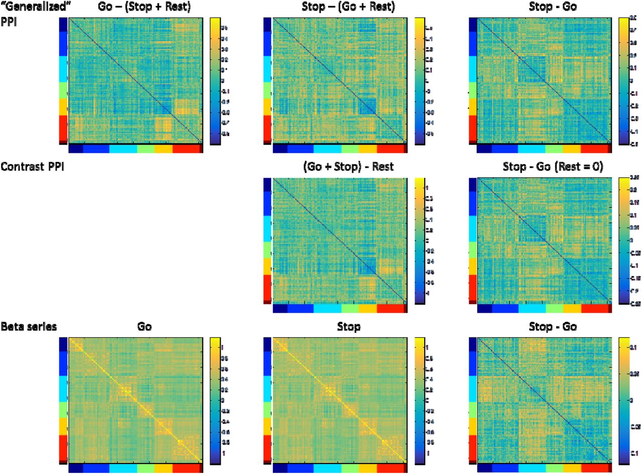
Psychophysiological interaction (PPI) and beta series correlation (BSC) results from the stop signal task. The top row showed the PPI matrices using the “generalized PPI” model, where the Go condition and Stop condition were modeled separately. The middle row showed the PPI matrices using direct contrast of the Go and Stop conditions. The bottom row showed correlation matrices using the beta series method. The right-side color scales of all matrices were made sure to be positive and negative symmetrical, but the range was adjusted based on the values in each matrix. The left and bottom color bars indicate the seven functional modules, including cerebellar, cingulo-opercular, default mode, frontoparietal, occipital, sensorimotor, and emotion modules from dark blue to dark red.

Scatter plots between the psychophysiological interaction (PPI) and beta series correlation (BSC) matrices. A shows the relationship between the Stop – Go contrasts calculated from the contrast and “generalize” PPI methods. B shows the relationship between the Go – baseline contrast from the “generalize” PPI analysis and the Go condition from the BSC analysis. C shows the relationship between the Stop – baseline contrast from the “generalize” PPI analysis and the Stop condition from the BSC analysis.

Resting-state functional connectivity matrix (mean Fisher’s z) from a subset of 103 subjects (A), and its relationship with the beta series correlations (BSC) matrices of single conditions (B and C).
The connectivity differences between the Stop and Go conditions have been reported previously (Di and Biswal, 2018). Here we only focus on the effect of task execution, i.e. the mean effect of the Go the Stop conditions compared with the baseline. Statistical significant effects were thresholded at p < 0.05 (FDR corrected) and visualized using BrainNet Viewer (Xia et al., 2013) (Figure 9). It clearly shows that there was reduced connectivity within the visual areas, and increased connectivity mainly between visual regions and sensorimotor regions and between visual regions and other brain regions such as cingulo-opercular regions.

Mean PPI effects of the Go and Stop trials compared with the implicit baseline. A shows the thresholded PPI matrix at p < 0.05 of FDR (false discovery rate) correction. Yellow represents positive PPI effects, while blue represents negative effects. The color bars indicate the seven functional modules, including cerebellar, cingulo-opercular, default mode, fronto-parietal, occipital, sensorimotor, and emotion modules from dark blue to dark red. B and C show the positive and negative effects on a brain model using BrainNet Viewer.
Lastly, for the contrast of Stop vs. Go where the two PPI models and BSC yielded similar results, we compared the BSC results with different methods with the PPI results (Figure 10). The significant effects of the “generalized PPI” and contrast PPI were identical. When comparing the three measures of Spearman’s correlation, Pearson’s correlation, and covariance, Pearson’s correlation produced more significant effects than Spearman’s correlation. And covariance differences only showed one positive and one negative significant effect. However, even the results from Pearson’s correlation showed less significant results than the two PPI models.

Unthresholded (upper row) and thresholded (lower row) matrices of task modulated connectivity between the Stop and Go conditions estimated by different methods. A p < 0.05 of false liscovery rate (FDR) correction was used to threshold each matrix. The color scales of all matrices were made sure to be positive and negative symmetrical. But the range was adjusted based on the values in each matrix.
4. Discussion
In the current paper, we have compared between PPI and BSC, and explained that because the inclusion of the physiological variable in the PPI model, a PPI effect always represents the differences of correlations between conditions. In contrast, BSC can measure correlations in a specific task condition. However, when comparing between conditions, PPI and BSC methods should in principle yield similar estimates of connectivity differences. The results of PPI and BSC analyses on a real event-related designed stop signal task agree with our theoretical explanation of the two methods. Firstly, PPI always conveyed connectivity differences between conditions, even when using a simple psychological variable of 1s and 0s. The direct contrast PPI could show exactly the same results as “generalized PPI” when the conditions were modeled properly. Secondly, we showed that simple correlations of beta series in one condition reflected the absolute effects of connectivity, which resembled resting-state connectivity. However, when the effects were contrasted between conditions, the PPI and BSC results turned out to be very similar.
The simple BSC correlation for the Go and Stop conditions are very similar to each other, and are also similar to what we typically observed in resting-state. They all show square like structures along the diagonal, which reflects higher functional connectivity within the predefined functional modules, and lower functional connectivity between regions from different functional modules. This is consistent with the observation that the moment-to-moment correlations in many different task conditions are very similar (Cole et al., 2014). On the other hand, for PPI analysis even the simple PPI effects of one condition yield connectivity differences between the very condition and the rest of the time points. In the current analysis, we demonstrate the task modulated connectivity of the Go and Stop conditions compared with their respective baseline. But this cannot be achieved by using the BSC method, because the implicit baseline conditions cannot be easily modeled in the BSC model.
The connectivity differences between the Go or Stop conditions compared with their respective baseline suggested changes of connectivity related to general task executions. This contrast revealed decreased connectivity between visual areas, and increased connectivity between visual areas and sensorimotor areas among other brain regions. The reduced connectivity within the visual areas during task execution compared with baseline is consistent with our previous studies using a set of different tasks (Di et al., 2017) as well as in a simple checkerboard task (Di and Biswal, 2017). However, in contrast to the reduced functional connectivity between visual and sensorimotor regions in the checkerboard task (Di and Biswal, 2017), the current results showed increased connectivity between the visual and sensorimotor regions. It is not surprising because the stop signal task requires the subjects to response to visual stimuli, therefore yielding increased functional coupling between visual and sensorimotor regions.
When directly comparing the differences between the Stop and Go conditions, all the PPI and BSC methods showed similar results. First, the “generalized PPI” and contrast PPI showed identical results. It is not surprising given that we have explained they are mathematically equivalent. Although we think that the “generalized PPI” is still a better strategy to model PPI effects, in some circumstances the direct contrast method may be useful. For example, if there are too many task conditions designed (say conditions A, B, C, D, E, and a baseline condition R), but eventually one is only interested in one contrast of A vs. B, there is no need to model PPI effects of all the five conditions separately. One can model the mean effects of A and B and the contrast effect between A and B, leaving all other conditions as 0. In this way, the direct contrast method is more flexible in terms of defining psychological variables and contrasts.
As has been reported in our previous paper, BSC differences can yield similar connectivity differences when compared between the Stop and Go conditions (Di and Biswal, 2018). In the current analysis, we further compared BSC differences results using Pearson’s correlation and covariance. The unthresholded matrices of the three connectivity measures were very similar. When performing statistical inferences using a p < 0.05 threshold of FDR correction, Pearson’s correlation yielded more statistical significant effects than Spearman’s correlation, while covariance could only show two statistical significant effects. Nevertheless, the numbers of statistical significant effects were all smaller than those in the PPI analyses. Mathematically, the PPI effect is more similar to the covariance differences between conditions than the other correlation measures. However, the covariance differences of beta series failed to convey as many significant results as the other correlations measures. It is probably due to the fact that the BSC model for the stop signal task is not reliable enough, so that there are large amounts of spurious trial-by-trial variability that need to be standardized before calculating covariance.
In this paper, we have explained the relationships between PPI and BSC, and showed that in principle these two methods should measure the same connectivity differences between conditions. However, PPI and BSC methods could yield slightly different results mainly due to the different ways of dealing with deconvolution or trail-by-trial activation estimates. Because of this, simply comparing the two methods is less of interest. Further studies may focus on deconvolution techniques such that the results of both PPI and BSC could improve. For example, more sophisticated filters could be used for deconvolution, e.g. cubature Kalman filtering (Havlicek et al., 2011). In addition, applying subject specific HRF (Pedregosa et al., 2015) may be helpful for both PPI and BSC methods. Lastly, the effectiveness of the two methods may also depend on the temporal distance of trials (Abdulrahman and Henson, 2016; Mumford et al., 2014; Visser et al., 2016). Although the current study showed that both of the methods could work for the fast event-related stop signal task, it is reasonable to speculate that these two methods may work better when trial distances are larger. The fitness of the two methods on different design parameters warrants further investigations.
Acknowledgement
This study is funded by NIH grants R01 AG032088 and R01 DA038895.
Reference


