

Abstract
Coordinate-based meta-analyses (CBMA) allow researchers to combine the results from multiple fMRI studies with the goal of obtaining results that are more likely to generalise. However, the interpretation of CBMA findings can be impaired by the file drawer problem, a type of publications bias that refers to studies that are carried out but are not published due to lack of significance. Using foci per contrast count data from the BrainMap database, we propose a zero-truncated modelling approach that allows us to estimate the prevalence of non-significant contrasts. We validate our method with simulations and real coordinate data generated from the Human Connectome Project. Application of our method to the data from BrainMap provides evidence for the existence of a file drawer effect, with the rate of missing contrasts estimated as at least 6 per 100 reported.
1 Introduction
Now over 25 years old, functional magnetic resonance imaging (fMRI) has made significant contributions in improving our understanding of the human brain function. However, the inherent limitations of fMRI experiments have raised concerns regarding the validity and replicability of findings (Farah, 2014). These limitations include poor test-retest reliability (Raemaekers, 2007), excess of false positive findings (Wager, 2009) and small sample sizes (Carp, 2012). Meta-analyses play an important role in the field of fMRI as they provide a means to address the aforementioned problems by synthesising the results from multiple experiments and thus draw more reliable conclusions. Since the overwhelming majority of authors rarely share the full data, coordinate-based meta-analyses (CBMA), which use the xyz coordinates (foci) of peak activations that are typically published, are the main approach for the meta-analysis of fMRI data.
As in any meta-analysis, the first step in a CBMA is a literature search. During this step investigators use databases to retrieve all previous work which is relevant to the question of interest (Normand, 1999). Ideally, this process will yield an exhaustive or at least representative sample of studies on a specific topic. Unfortunately, literature search is subject to the file drawer problem (Rosenthal, 1979; Iyengar and Greenhouse, 1988). This problem refers to research studies that are initiated but are not published due to lack of significance, either by cause of authors’ hesitation to submit or perhaps because of rejection by journals that are reluctant to publish negative results. The file drawer along with the other forms of publication bias (see Song et al. (2000) for an overview) can potentially undermine the quality of a meta-analysis as they lead to biased estimates of the effect of interest (Begg and Berlin, 1988; Sutton, 2000). Aside from distorting a particular scientific question of interest, this feeds into researchers’ scepticism regarding the usefulness of meta-analysis (Greenland, 1994).
Evidence of the file drawer problem has been found in many fields of scientific research, including psychology (Kuhberger et al., 2014), public health (Dwan, 2008, 2013) and the social sciences (Sterling, 1995). Therefore, several methods have been proposed for detecting and sometimes adjusting for the presence of the file drawer problem. Early literature was focused on finding the fail-safe N (Rosenthal, 1979; Iyengar and Greenhouse, 1988), the minimum number of unpublished studies required to overturn the outcome of meta-analysis. Much attention has been given to the graphical tool known as the funnel plot (Light and Pillemar, 1984; Egger, 1997), as well as methods that formalise this idea (Duval and Tweedie, 2000a,b, among others). Another very common approach involves the use of weight functions where the probability of observing a study is modelled as a function of its characteristics such as p-values, see e.g. Larose and Dey (1998); Copas and Jackson (2004). Finally, another popular approach is sensitivity analysis where one chooses a parametric model for the probability that an initiated body of research results in publication, and the outcome of meta-analysis is studied under different parameter values of the model (Copas, 1999, 2013). For an overview and more detailed description of methods for modelling the file drawer problem we refer the reader to Jin et al. (2015).
Since most of the aforementioned methodologies cannot be directly applied to fMRI coordinate-based meta-analysis data, there has been little investigation into potential biases in the field. One effort is Jennings and Van Horn (2012) that found evidence for publication biases in 74 studies of tasks involving working memory. The authors use the maximum test statistic reported in the frontal lobe as the effect estimate in their statistical tests. Another example is David et al. (2013), who studied the relation between sample size and the total number of activations and reached similar conclusions as Jennings and Van Horn (2012), finding publication bias mainly affecting small studies. However, to date there has been no work on estimating the fundamental file drawer quantity, that is the number of missing studies.
In what follows, we propose a model for estimating the prevalence of nonsignificant contrasts omitted from a large cohort of studies in the context of CBMA. The remainder of the paper is organised as follows. In Section 2, we describe the CBMA data, both real and simulated, that we used and the statistical model for point data that accounts for missing studies. In Section 3, we present the results of our simulation studies and real data analyses. Finally, in Section 4 we conclude with a discussion of our main findings and set directions for future research.
2 Methods
2.1 BrainMap database
Our analysis is motivated by coordinate data from BrainMap 1 (Laird, 2005). BrainMap is an online, freely accessible database for coordinate-based data of both functional and structural neuroimaging experiments. The database is continuously expanding and as of November 2014 consists of results obtained from 2,562 scientific papers, each one of these containing several experiments or contrasts. BrainMap is a widely used resource, and many meta-analyses are based on data retrieved from this database (see Hill et al. (2014) and Kirby and Robinson (2015) for some recent examples). It is therefore of vital importance to investigate the presence of the file drawer problem and its possible effects on meta-analysis.
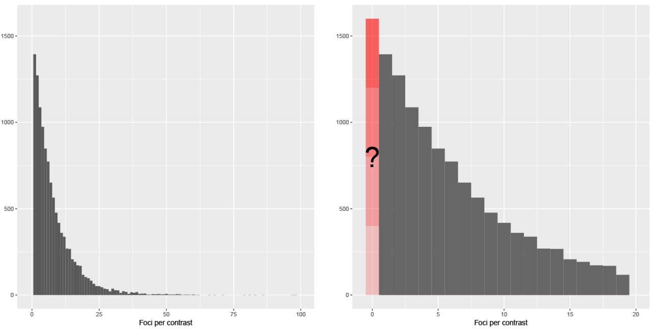
Our unit of observation is a contrast, and hence our dataset consists of 12,292 observations. Each observation (contrast) consists of a list of three dimensional coordinates xi, the foci, typically either local maxima or centers of mass of voxel clusters with significant activations. For the purposes of this work we ignore the spatial aspect of the problem and instead model the file drawer only based on the the total number of foci per contrast ni. Further, we do not consider any of the resting-state studies that are registered in BrainMap. Table 1 presents presents some summary statistics of the BrainMap dataset, whereas Figure 1 shows the empirical distribution of the total number of foci per contrast.
BrainMap database summaries.

Empirical distribution of the total number of foci per contrast in the BrainMap database, ni. The left panel shows the full distribution, while the right panel shows a zoomed-in view of all studies reporting 24 or fewer foci. The BrainMap database does not record incidents of null contrasts (contrasts in a study for which ni = 0).
The barplot of Figure 1 (right) identifies a fundamental aspect of this data: even though the distribution of ni has most of its mass close to zero, there are no contrasts with zero foci. Thus we are careful not to describe our estimates as ‘null study’ prevalence. Rather, we are estimating prevalence of null contrasts, some of which may in fact be clearly reported in papers in the BrainMap database; however, given the stigma of negative findings, we suspect these type C null contrasts are rare.
2.2 Models
Our model uses count data from the observed, reported experiments to infer on the file drawer quantity. At this point, we make some critical assumptions: I) data  , both observed and unobserved, are taken to be independent and identically distributed (i.i.d.) samples from a count distribution N of a given parametric form (we will relax this assumption later, to allow for inter-study covariates); II) the probability of publication depends on the total number of significant activations ni; specifically, this probability equals zero for experiments with ni = 0 and equals one for studies with ni ≥ 1. For a detailed discussion of the implications of assumptions I-II, see Section 4.
As each paper in the BrainMap database has multiple contrasts, potentially violating the independence assumption, we draw subsamples such that exactly one contrast from each publication is used. Specifically, we create 5 subsamples (A-E) drawing 5 different contrasts for each subsample, if possible; for publications with less than 5 contrasts we ensure that every contrast is used in at least one subsample, and then randomly select one for the remaining subsamples.
If assumptions I-II described above hold, then a suitable model for the data is a zero-truncated count distribution. A zero-truncated count distribution occurs when we restrict the support of a count distribution to the positive integers. For a probability mass function (pmf) π (n | θ) defined on n = 0, 1,…, where θ is the parameter vector, the zero truncated pmf is:

We consider three types of count distributions π (n | θ): the Poisson, the Negative Binomial and the Delaporte. The Poisson is the classic distribution for counts arising from series of independent events. In particular, if the foci in a set of experiments arise from a spatial Poisson process with common intensity function, then the resulting counts will follow a Poisson distribution. Poisson models often fit count data poorly due to over-dispersion, that is, the observed variability of the counts is higher than what would be anticipated by a Poisson distribution. More specifically, if a spatial point process has a random intensity function, one that changes with each set of observed points, the distribution of counts will show this over-dispersion. In particular, we note that in our previous work (Kang, 2011) we have always used such ‘Cox processes’ with random intensity functions.
The Negative Binomial distribution is the count distribution arising from the Poisson-Gamma mixture: if the true Poisson rate differs between experiments and is distributed as a Gamma random variable, then the resulting counts will follow a Negative Binomial distribution. For the Negative Binomial distribution we use the mean-dispersion parametrisation:
 where μ is the mean, ϕ > 0 is the dispersion parameter and Γ (·) represents the gamma function; with this parametrisation the variance is
  . Hence, the excess of variability compared to the Poisson model is accounted for through the additional term
  .
.
The Delaporte distribution is obtained by modelling the foci counts ni of experiment i as Pois(μγi) random variables; the γi follows a particular shifted Gamma distribution with parameters σ and ν, σ > 0 and 0 ≤ ν < 1 (Rigby, 2008). The probability mass function of the Delaporte distribution can be written as:
 where μ is the mean and:

With this parametrisation the variance of the Delaporte distribution is μ + μ2σ(1 − ν)2.
Once the parameters of the truncated distribution are estimated, one can make statements about the original, untruncated distribution. One possible way to express the file drawer quantity is the percent prevalence of zero count contrasts pz, that is, the total number of missing experiments per 100 published. This can be estimated as:

Here,  denotes the probability of observing a zero count contrast, and
  denotes the estimated parameter values from the truncated model (e.g. θ = (μ, σ, ν)⊤ for the Delaporte model).
Our statistical model is based on homogenous data, and we can reasonably expect that differences in experiment type, sample size, etc., can introduce systematic differences between studies. To explain as much of this nuisance variability as possible, we further model the expected number of foci per experiment as a function of its characteristics in a log-linear regression:
 where xi is the vector of covariates and β is the vector of regression coefficients. The covariates that we consider are: i) the year of publication ranging from 1985 to 2014 with median 2004; ii) the square root of the number of participants ranging from 1 to 395 with median 12; iii) the experimental context. For experimental context we use 7 levels: age effects, disease effects, drug effects, gender effects, learning, linguistic effects, normal mapping and other. The first six levels appeared at least 20 times in the database while ‘other’ covers any other label that occured less frequently. Even though the BrainMap database records multiple labels for each experiment, we only used the first one. Summaries of the BrainMap subsamples A-E data for each level of context can be found in A.
Parameter estimation is done under under the generalized additive models for location scale and shape (GAMLSS) framework of Rigby and Stasinopoulos (2005). The fitting is done in R2 (R Core Team, 2015) with the gamlss library (Stasinopoulos and Rigby, 2007). Confidence intervals are obtained with the bootstrap. When covariates are included in the model, we use the stratified bootstrap to ensure representation of all levels of the experimental context variable. In particular, for each level of the categorical variable a bootstrap subsample is drawn using the data available for this class and subsequently these subsamples are merged to provide the bootstrap dataset. Model comparison is done using the Akaike information criterion (AIC) provided by the package.
2.3 Monte Carlo evaluations
We perform a simulation study to assess the quality of estimates of pz, the total number of experiments missing per 100 published, obtained by the zero-truncated Negative Binomial and Delaporte models (initial work found Brain-Map counts completely incompatible with the Poisson model, and hence we did not consider it for simulation). For both approaches, synthetic data are generated as follows. First, we fix the values of the parameters, that is, μ, ϕ for the Negative Binomial distribution and μ, σ, ν for the Delaporte distribution. We then generate  samples from the untruncated distributions, where I* is chosen such that the expected number of non-zero counts is I. We remove the zero-count instances from the simulated data and the corresponding zero-truncated model is fit to the remaining observations. Finally, we estimate the probability of observing a zero count experiment based on our parameter estimates.
We set our simulation parameter values to cover typical values found in BrainMap (see C, Table 8). For the Negative Binomial distribution we consider values 4 and 8 for the mean and values 0.4, 0.8, 1.0 and 1.5 for the dispersion, for a total of 8 parameter settings. For the Delaporte distribution, we set μ to 4 and 8, σ to 0.5, 0.9 and 1.2, and ν to 0.02, 0.06 and 0.1 (18 parameter settings). The expected number of observed studies is set to I = 200, 500, 1,000 and 2,000. For each combination of (I, μ, ϕ) and (I, μ, σ, ν) of the Negative Binomial and Delaporte models, respectively, we generate 1,000 datasets from the corresponding model, for each parameter setting, and record the estimated value of pz for each fitted dataset.
2.4 HCP real data evaluations
As an evaluation of our methods on realistic data for which the exact number of missing contrasts is known, we generate synthetic meta-analysis datasets using the Human Connectome Project task fMRI data. We start with a selection of 80 unrelated subjects and retrieve data for all 86 tasks considered in the experiment. For each task, we randomly split the 80 subjects into 8 groups of 10 subjects. Hence, we obtain a total of 86 × 8 = 688 synthetic fMRI experiments. For each experiment, we perform a one-sample group analysis, using ordinary least squares in FSL3, and recording  , the total number of surviving peaks after random field theory thresholding at the voxel level, 1% familywise error rate (FWE), where i = 1,…, 688. We also record the total number of peaks (one peak per cluster) after random field theory thresholding at the cluster level, cluster forming threshold of uncorrected P=0.00001 & 1% FWE,
  . These rather stringent significance levels were needed to induce sufficient numbers of results with no activations. We then discard the zero-count instances from
  and
and  , and subsequently analyse the two truncated samples in two separate analyses, using the zero-truncated Negative Binomial and Delaporte models. Finally, the estimated number of missing experiments is compared to the actual number of discarded contrasts. Note that we repeat the procedure described above 6 times, each time using different random splits of the 80 subjects (HCP splits 1-6).
3 Results
3.1 Simulation results
The percent relative bias of the estimates of  , and its bootstrap standard error for the zero-truncated Negative Binomial and Delaporte models are shown in Table 2 and Table 3, respectively. The results indicate that, when the model is correctly specified, both approaches perform adequately. In particular, in Table 2 we see that the bias of
  is small, never exceeding 8% when the sample size is comparable to the sample size of the BrainMap database (I = 2, 555) and the mean number of foci is similar to the average foci count found in BrainMap (≈ 9). The bootstrap standard error estimates produced by the Negative Binomial model are also accurate with relative bias below 5% in most scenarios with more than 500 contrasts, while Delaporte tends to underestimate standard errors but never more than-15% (see Table 3).
Percent relative bias for estimation of pz, the zero-count experiment rate as a percentage of observed studies, for Negative Binomial and Delaporte models as obtained from 1,000 simulated datasets. Parameter μ is the expected number of foci per experiment, ϕ, σ and ν are additional scale and shape parameters. Negative Binomial performs well and, while Delaporte often underestimated pz, with at least 1,000 contrasts it always has bias less than 10% (positive bias over-estimates the file drawer problem).
Percent relative bias of bootstrap standard error of  , missing experiment rate as a percentage of observed studies, for Negative Binomial and Delaporte models as obtained from 1,000 simulated datasets. Parameter μ is the expected number of foci per experiment and ϕ, σ and ν are additional scale and shape parameters. For a sample of at least 1,000 contrasts, Negative Binomial standard errors are usually less than 3% in absolute value; while Delaporte has worse bias, it is never less than −15% (negative standard error bias leads to over-confident inferences).
3.2 HCP synthetic data results
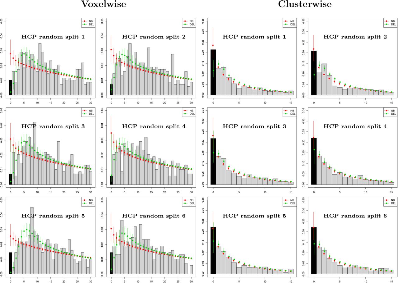
Results of the analysis of the HCP synthetic datasets using the zero-truncated Negative Binomial and Delaporte models are summarised in Figure 2 and Table 4. In Figure 2 we plot the empirical count distributions and the fitted probability mass functions for the 12 datasets considered. For datasets obtained with voxelwise thesholding of the image data, we see that the Delaporte distribution provides a better fit compared to the Negative Binomial qualitatively, and by AIC for all 6 datasets (Table 4). For clusterwise thresholding, there are fewer peaks in general and their distribution is less variable compared to voxelwise thresholding. Both distributions achieve a similar fit. Here, AIC supports the Negative Binomial model in 4 out of 6 datasets.

Evaluation with HCP data with 688 contrasts of sample size 10, comparing accuracy of Negative Binomial (NB) and Delaporte (DEL) distributions for the prediction of the number of studies with no significant results (zero foci) based on only significant results (one or more foci). Left panel shows results for voxelwise inference, right for clusterwise inference, both using PFWE=0.01 to increase frequency of zero foci. For clusterwise datasets, the Negative Binomial confidence intervals always include the observed zero count, while Delaporte ofter underestimates the count. For voxelwise analysis, the Negative Binomial over-estimates the zero frequency substantially, while Delaporte’s intervals include the actual zero frequency in 3 out of 5 splits.
Evaluation of the zero-truncated modeling approach using synthetic data obtained from the HCP project, using voxelwise (top) and clusterwise (bottom) inference. The true number of missing contrasts (n0) for each one of the 12 datasets (6 for voxelwise thesholding and 6 for clusterwise thresholding) is shown in the second column. For each of the Negative Binomial and Delaporte methods, the estimated missing contrast count (n0), 95% bootstrap confidence interval for n0 and AIC score are shown (smaller AIC is better).
Table 4 reports the true number of missing contrasts n0, along with point estimates  and the 95% bootstrap intervals obtained by the zero-truncated models. For voxelwise data, the Negative Binomial model overestimates the total number of missing experiments in all 6 datasets as a consequence of the poor fit to the non-zero counts, while the Delaporte model bootstrap intervals include the true value of n0 in 5 out of 6 datasets, greatly underestimating n0 in one dataset. For clusterwise counts, the point estimates obtained by the zero-truncated Negative Binomial model are very close to the true values. Notably, n0 is included within the bootstrap intervals for all 6 datasets. The Delaporte model underestimates the values of n0 in all 6 datasets, but the bootstrap intervals include n0 for 4 out of 6 datasets.
Overall, we find that the zero-truncated modeling approach generally provides good estimates of n0, with the Negative Binomial sometimes overestimating and the Delaporte sometimes underestimating n0. A conservative approach, therefore, favors the Delaporte model.
3.3 Application to the BrainMap data
We found the Poisson distribution to be completely incompatible with the Brain-Map count data (B, Figure 6), and we do not consider it further. We start by fitting the Negative Binomial and Delaporte zero-truncated models without any covariates. Figure 3 shows the emprical and fitted probability mass functions for the 5 subsamples. We see that both distributions provide a good fit for the BrainMap data. The Negative Binomial model is preferred based on AIC in 4 out of 5 but with little difference in AIC (Table 6). The estimated prevalence of missing contrasts, along with 95% bootstrap intervals are shown in Table 5. Note that while there is considerable variation in the estimates over the two models, the confidence intervals from all subsamples do not include zero, thus suggesting a file drawer effect.

BrainMap results for 5 random samples using the Negative Binomial and Delaporte models and no covariates. Plots show observed count data (gray bars) with fit of full (non-truncated) distribution based on zero-truncated data, including the estimate of p0 (over black bar).
BrainMap data analysis results. The table presents the estimated prevelance of file drawer studies along with 95% bootstrap confidence intervals, as obtained by fitting the zero-truncated Negative Binomial and Delaporte models to BrainMap subsmaples A-E. No covariates are considered.
AIC model comparison results for the BrainMap data. The AIC is found by fitting the zero-truncated Negative Binomial and Delaporte models, with and without the covariates, to BrainMap subsamples A-E. Every split indicates evidence for better fit with covariates (smaller AIC indicates better fitting model).
Covariates essentially have no effect on the estimated prevalence of missing contrasts. However, including covariates results in an improvement in terms of AIC for both models and all BrainMap subsamples (Table 6). As can be seen in Figure 4, the estimated prevalence of zero count contrasts is a slowly decreasing function of both the square root number of participants and the year of publication. For the former, the trend is expected and one possible explanation is that bigger samples result into greater power, and therefore more foci and thus less of a file drawer problem. However, for publication year, decreasing publication bias is welcomed but we could have just as well expected that the increased use of multiple testing in later years would have reduced foci counts and increased the file drawer problem. Finally, we see that the estimated percent prevalence of zero-count contrasts is similar for all levels of the categorical variable context, with the exception of experiments studying gender effects (Figure 5).
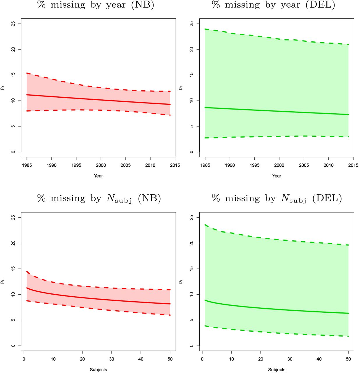
Predicted pz, missing experiment rate per 100 published experiments, as a function of year of publication (top) and the square root of sample size (bottom), with pointwise 95% bootstrap confidence intervals. There is not much variation in the estimate of the percentage missing, but in both cases a negative slope is observed, as might be expected with improving research practices over time and greater power with increased sample size. All panels refer to the first BrainMap random sample (subsample A).
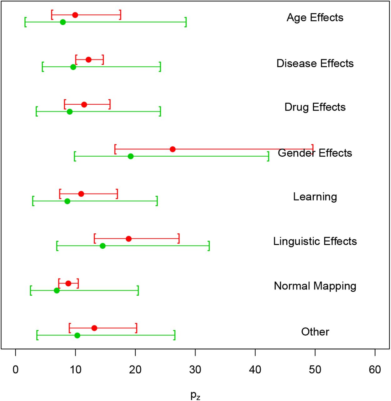
Studies missing per 100 published as a function of experiment context, with 95% bootstrap confidence intervals. Note that we have fixed the year and square root sample size covariates to their median values. The plot is derived from the first BrainMap random sample (subsample A).
4 Discussion
Summary
In this paper, we have proposed a method for estimating the total number of contrasts missing from a large cohort of CBMA studies due to the file drawer problem. Our method uses intrinsic statistical characteristics of the non-zero count data to infer zero counts. This is achieved by estimating the parameters of a zero-truncated model, either Negative Binomial or Delaporte, which are susequently used to predict the prevalence p0 of zero-count studies in the original, untruncated distribution, and re-expressing this as pz, the rate of missing contrasts per 100 published. The approach relies on assumptions I and II described in Section 2.2. Assumption I implies that there is independence between contrasts. However, as one publication can have several contrasts, this assumption is tenuous despite it being a standard assumption for most CBMA methods. To ensure the independence assumption is valid, we subsample the data so that only one randomly selected contrast per publication is used. Assumption II defines our censoring mechanism, such that experiments with at least one significant activation are always published. The assumption that nonsignificant research findings are suppressed from the literature has been adopted by authors in classical meta-analysis (Eberly and Casella, 1999, among others) and we believe that is reasonable in the context of CBMA as well.
A series of simulations studies suggest that the zero-truncated modelling approach provides valid estimates of the file drawer quantity. A critical limitation of our HCP evaluation is the repeated measures structure, where 86 contrasts come from each subject. Such dependence generally does not induce bias in the mean estimates, but can corrupt standard errors and is a violation of the bootstrap’s independence assumption. However, as the bootstrap intervals generally captured the true censoring rate, it seems we were not adversely affected by this violation. It should be noted, moreover, that the properties of our estimators degrade as the total number of observed studies decreases and therefore the methods should not employed for meta-analyses with a small number of studies, below, say, 1,000 studies.
We find that both zero-truncated Negative Binomial and Delaporte models provide a good fit for the total number of foci per contrast in the BrainMap database. The analysis suggests that the estimated magnitude of the file drawer slightly varies depending on study characteristics, but generally consists of at least 6 missing experiments for 100 published and is significantly greater than zero.
Implications for meta-analyses
Our findings provide evidence for the existence of publication bias in CBMA. While we cannot rule out a contribution of contrasts that have actually been reported in the original publications and not encoded in the database, we posit that the majority come from contrasts never described in publications or not published at all.
We stress that this analysis is totally agnostic to the statistical procedures used to generate the results in the BrainMap database. The counts we model could have been found with liberal P < 0.001 uncorrected inferences or stringent P < 0.05 FWE procedures. However, if the neuroimaging community never used multiple testing corrections, then every experiment should report many peaks, and we should estimate virtually no missing studies. In the end, our results reflect the aggregate statistical practice and signal structure reflected in the BrainMap database.
Ideally, our unit of inference would be a publication. However, linking our contrast-level inferences to studies requires assumptions about dependence of contrasts within a study and the distribution of the number of contrasts examined per study. We can assert that the more contrasts examined per investigation, the more likely 1 or more null contrasts should arise; and that the risk of null contrasts is inversely related to foci-per-contrast of non-null contrasts.
The presence of missing experiments does not invalidate existing studies, but complements the picture seen when conducting a literature review. Nevertheless, there are some implications concerning the interpretation of the results obtained from current CBMA approaches. In particular, methods that make no adjustments for the file drawer effect are conditional on the existence of at least one activation. Hence, effect estimates obtained trough a CBMA are inflated unless the prevalence of null exeriments is zero.
Future work
The analysis conducted in this paper is based on data retrieved from a single database. As a consequence, results are not robust to possible biases in the way publications are included in this particular database. A more thorough analysis would require consideration of other databases (e.g. Neurosynth.org4 (Yarkoni, 2011), though note Neurosynth does not report foci per contrast but per paper). Secondly, one may argue that our censoring mechanism is rather simplistic, and does not reflect the complexity of current (and potentially) poor scientific practice. For example, we have not allowed for the possibility of ‘vibration effects’, that is, changing the analysis pipeline (e.g., random vs fixed effects, linear vs. nonlinear registration) to finally obtain some significant activations. This would be an instance of initially-censored (zero-count) data being ‘promoted’ to a non-zero count through some means. Such models can be fit under the Bayesian paradigm and will be examined in our future work.
A BrainMap summaries for study context
In this section we provide summaries of the data on the 5 BrainMap subsamples A-E, for the different levels of the categorical variable study context. In particular, Table 7 presents the total number of studies per level, the average sample size per contrast, and the average number of foci per contrast. Note that in subsamples C and E there were less than 20 contrasts with label ‘Gender effects’; hence, we incorporate those in the ‘Other’ category.
Data summaries for the different levels of the categorical variable study context.
B Zero-truncated Poisson analysis of the Brain-Map dataset
In this section, we present results of the analysis of BrainMap subsamples A-E using the zero-truncated Poisson model. The empirical and fitted Poisson probability mass functions are shown in Figure 6. It is evident that the zero-truncated Poisson model provides a poor fit to the BrainMap data. The finding is confirmed by the AIC criterion which is 26067.2, 25303.4, 26006.6, 25018.8 and 25507.7 for subsamples A-E, respectively. These values are much higher than the corresponding values obtained by fitting both the Negative Binomial and Delaporte models (see Table 6). The estimated prevalence of file drawer studies is estimated as almost zero in all subsamples (Figure 6, final plot). However, these estimates should not be trusted considering the poor fit provided by the zero-truncated Poisson model.

BrainMap results for 5 random samples using the zero-truncated Poisson distribution. The first 5 plots show observed count data (gray bars) with fit of full (non-truncated) distribution based on zero-truncated data, including the estimate of p0 (over black bar). Final plot shows estimates of pz, prevalence of file drawer studies for every 100 studies observed. All fitted values include 95% bootstrap confidence intervals. The Poisson model provides a poor fit to all 5 subsamples.
C Negative Binomial and Delaporte parameter estimates
In this section, we present the parameter estimates obtained from the analysis of BrainMap subsamples A-E with the simple (without covariates) zero-truncated Negative Binomial and Delaporte models. The parameter estimates are listed in Table 8.
Scalar parameter estimates obtained when fitting the simple zero-truncated Negative Binomial and Delaporte models to BrainMap subsamples A-E.
Acknowledgements
The authors are grateful to Daniel Simpson, Paul Kirk and Solon Karapanagiotis for helpful discussions. This work was largely completed while PS, SM and TEN were at the University of Warwick, Department of Statistics. PS, TDJ and TEN were supported by NIH grant 5-R01-NS-075066; TEN was supported by a Wellcome Trust fellowship 100309/Z/12/Z and NIH grant R01 2R01EB015611-04. The work presented in this paper represents the views of the authors and not necessarily those of the NIH or the Wellcome Trust Foundxation.


