

Abstract
The accuracy of microbial community surveys based on marker-gene and metagenomic sequencing (MGS) suffers from the presence of contaminants — DNA sequences not truly present in the sample. Contaminants come from a variety of sources, including reagents. Appropriate laboratory practices can reduce contamination in MGS data, but do not eliminate it. Here we introduce decontam (https://github.com/benjjneb/decontam), an open-source R package which implements a statistical classification procedure for identifying contaminants in MGS data. Contaminants are identified on the basis of two widely reproduced signatures: contaminants are more frequent in low-concentration samples, and are often found in negative controls. In a dataset from the human oral microbiome, the classification of amplicon sequence variants by decontam was strongly consistent with prior microscopic observations of microbial taxa in that environment. In both metagenomics and marker-gene measurements of a mock community dilution series, the removal of contaminants identified by decontam substantially reduced technical variation due to differences in reagents and sequencing centers. The application of decontam to two recently published datasets corroborated and extended their conclusions that little evidence existed for an indigenous placenta microbiome, and that some low-frequency taxa seemingly associated with preterm birth were run-specific contaminants. decontam integrates easily with existing MGS workflows, and allows researchers to generate more accurate profiles of microbial community composition at little to no additional cost.
Introduction
High-throughput sequencing of DNA from environmental samples is a powerful tool for investigating microbial and non-microbial communities. Community composition can be characterized by sequencing taxonomically informative marker genes, such as the 16S rRNA gene in bacteria (Fox et al. 1980, Eckburg et al. 2005, Turnbaugh et al. 2009, Ravel et al. 2011). Shotgun metagenomics, in which all DNA recovered from a sample is sequenced, can also characterize functional potential (Riesenfeld et al. 2004, Gill et al. 2006, Anantharaman et al. 2016). However, the accuracy of marker-gene and metagenomic sequencing (MGS) is limited in practice by several processes that introduce contaminants into the data, i.e. artefactual DNA sequences that are not truly present in the sampled community.
Failure to account for DNA contamination can result in inaccurate data interpretation. Contamination falsely inflates within-sample diversity (Jervis-Bardy et al. 2015, Jousselin et al. 2015), obscures differences between samples (Adams et al. 2015, Jervis-Bardy et al. 2015), and interferes with comparisons across studies (Adams et al. 2015, Sinha et al. 2015). Contaminating DNA competes with sample DNA for PCR and sequencing reagents (Salter et al. 2014). In samples with less endogenous sample DNA, contaminants are more likely to comprise a significant fraction of sequencing reads (Glassing et al. 2016). As a result, DNA contamination disproportionately affects samples from low-biomass environments (Riley et al. 2013, Salter et al. 2014, Lauder et al. 2014, Lusk 2014, Adams et al. 2015), and can lead to controversial claims about the presence of bacteria in low microbial biomass environments like blood and body tissues (Riley et al. 2013, Aagaard et al. 2014, Lusk 2014, Lauder et al. 2016, Glassing et al. 2016). In high-biomass environments, contaminants can comprise a significant portion of the low-frequency sequences in the data (Edgar 2016), limiting reliable resolution of low-frequency variants and contributing to false-positive associations in exploratory analyses (Callahan & DiGiulio et al. 2017).
Attempts to control DNA contamination before and after sequencing have had mixed success. One common practice is to process reagent-only (Salter et al. 2014, Jousselin et al. 2014) or blank sampling instrument (Bittinger et al. 2014) negative control samples alongside biological samples at the DNA extraction and PCR steps. Contamination is often assumed to be absent if control samples do not yield a band on an agarose gel (e.g. Herrera & Cockell 2007, Koren et al. 2011). However, samples that contain DNA concentrations too low to be visualized by gel electrophoresis still generate non-negligible numbers of sequencing reads (Salter et al. 2014, Lauder et al. 2016), which suggests that gel-based quality control is insufficient.
There are multiple sources of contaminating DNA in MGS experiments. These include research subjects’ or investigators’ bodies (Kitchin et al. 1990, Meadow et al. 2015), sample collection instruments and laboratory reagents (Salter et al. 2014, Jousselin et al. 2015, Glassing et al. 2016), laboratory surfaces and air (Knights et al. 2011, Bittinger et al. 2014, Adams et al. 2015), and other samples within the same sample processing cohort (Jousselin et al. 2015). Investigators can reduce the impact of some of these sources of contamination through laboratory techniques such as UV irradiating reagents and lab surfaces, enzymatically treating reagents, the use of “ultrapure” reagents, and separating pre- and post-PCR areas (Rand et al. 1990, Patel et al. 2012, Jousselin et al. 2015, Glassing et al. 2016). However, adherence to these recommended lab practices reduces, but does not eliminate, DNA contamination (Salter et al. 2014, Sinha et al. 2015).
In silico removal of contaminants after sequencing complements laboratory approaches to reducing contamination. However, distinguishing contaminating microbial DNA from microbial sequences truly present in the sampled community (Salter et al. 2014, Lusk 2014) can be difficult, and most researchers do not use in silico methods to identify and remove DNA contaminants present in datasets after sequencing. Perhaps the most common in silico decontamination method is the removal of sequences that fall below an ad hoc abundance threshold (Flores et al. 2010, Bittinger et al. 2014, Willner et al. 2012, Lazarevic et al. 2016). However, the removal of rare sequences also removes rare features truly present in the sample, and fails to remove abundant contaminants that are most likely to interfere with subsequent analysis. Another approach is the removal of sequences that appear in negative controls (e.g. Dunn et al. 2013, Adams et al. 2015). However, this approach is often too stringent because cross-contamination between samples causes abundant true sequences to be detected in negative controls (Callahan & DiGiulio et al., 2017, Jousselin et al. 2015). Finally, some investigators implement blacklist methods, which exclude sequences or taxa that have been previously identified as contaminants. This approach can be useful, but fails to identify rare or study-specific contaminants, and removes true members of the sampled community that overlap with previously observed contaminants.
To our knowledge, only two software tools have been developed that directly address the problem of contamination in MGS data. SourceTracker uses Bayesian mixture models to identify the proportion of a sample that is consistent with origin from a contaminating source of known composition, but does not identify specific contaminant sequences (Knights et al. 2011). A workflow in the An’vio software package leverages the visualization and summary statistics provided by An’vio to better partition metagenomic data into genomic bins and identify contaminant metagenome-assembled-genomes (MAGs) (Delmont & Eren 2016), but does not apply to marker-gene data and relies on user expertise to identify contaminant-specific patterns.
Here, we introduce decontam, a simple-to-use and open-source R package that identifies and removes contaminants in MGS data. decontam implements two simple statistical tests based on widely reproduced signatures of contamination: (1) Sequences from contaminating taxa are likely to have frequencies that inversely correlate with sample DNA concentration (Willner et al. 2012, Lusk 2014, Salter et al. 2014, Jervis-Bardy et al. 2015), and (2) sequences from contaminating taxa are likely to have higher prevalence in control samples than in true samples (Dunn et al. 2013, Adams et al. 2015, Lazarevic et al. 2016). Detection of these signatures can be readily integrated with current best practices. Frequency-based contaminant identification relies on auxiliary data from DNA quantitation that is in most cases intrinsic to MGS sample preparation, while prevalence-based contaminant identification relies on data from sequenced negative controls, a recommended practice in MGS studies (Salter et al. 2014, Sinha et al. 2015) that can be easily and cheaply performed.
We validated decontam on marker-gene and metagenomics datasets generated by our laboratory and others. In an oral 16S rRNA gene dataset, decontam identified low- and high-frequency contaminants consistent with curated databases of common contaminating microbial genera and known oral microbes. In data generated by Salter et al., the removal of contaminants identified by decontam reduced technical variation due to sequencing center in marker-gene data, and reduced technical variation due to DNA extraction kit in shotgun metagenomics data. The application of decontam to data generated by Lauder et al. corroborated their conclusion that there was no evidence for a placenta microbiome in their 16S rRNA gene sequencing data. Finally, decontam improved the exploratory analysis of associations between preterm birth and the vaginal microbiota by removing run-specific contaminants from the marker-gene data analyzed in a recent study (Callahan & DiGiulio et al. 2017). Our results suggest that decontam can improve the accuracy of biological inferences across a wide variety of studies that use MGS methods to investigate microbial communities.
Description of the Method
The decontam R package
decontam is implemented as an open-source R package available from github (https://github.com/benjjneb/decontam), and in the future from the Bioconductor repository (Gentleman et al. 2004). The primary function, isContaminant, uses frequency- and/or prevalence-based patterns across samples to identify contaminant sequence features derived from marker-gene or metagenomics sequencing data. Valid sequence features include amplicon sequence variants (ASVs), operational taxonomic units (OTUs), taxonomic groups or phylotypes (e.g. genera), orthologous genes, metagenome-assembled-genomes (MAGs), and any other derived feature with a quantitative per-sample abundance.
The primary input to isContaminant is a feature table describing the quantitative abundance of sequence features across samples (e.g. an OTU table). In addition, isContaminant requires one of two types of sample metadata for frequency- and prevalence-based contaminant identification, respectively: (1) A vector of DNA concentrations for each sample, often obtained in the form of a fluorescence intensity (e.g. PicoGreen), or (2) a defined set of sequenced negative control samples, preferably DNA extraction controls to which no sample DNA was added. Contaminants identified by decontam can then be removed with basic R functions.
Frequency-based contaminant identification
Total DNA (T) in a sample is assumed to consist of a mixture of contaminating DNA (C) that is present in uniform concentration across samples (Salter et al. 2014, Lazarevic et al. 2016, Lauder et al. 2016) and true sample DNA (S) that is present in varying concentration across samples. In the limit of S >> C, the frequency of contaminating DNA (fC) is inversely proportional to the total DNA (Jervis-Bardy et al. 2015, see also Fig. 1a), while the frequency of true sample DNA (fS) is independent of total DNA:


(a) Theoretical frequencies of sequences across samples; expected contaminant frequency varies inversely with sample DNA concentration (red), while expected non-contaminant frequency does not (blue). (b) Theoretical prevalence of multiple contaminant and noncontaminant sequences in samples and negative controls. Sequences below the dotted line are more prevalent in controls than true samples, and are likely contaminants.
Sequence features are classified by comparing a “contaminant” model, in which expected feature frequency is constrained to vary inversely with total DNA concentration, to a “noncontaminant” model, in which expected feature frequency is constrained to be independent of total DNA concentration. More precisely, two linear models of the log-transformed frequencies as a function of the total DNA concentration are fit over all samples in which the feature is present, a contaminant model with the slope set to -1 and a non-contaminant model with the slope set to 0. An F statistic is computed from the ratio between the sums-of-squares of the residuals of the contaminant model and the non-contaminant model, and then the tail probability that a small or smaller F statistic would have occurred by chance is calculated. Small probabilities indicate that the contaminant model is a significantly better fit than the noncontaminant model.
When contaminants comprise a large fraction or majority of sequencing reads (i.e. C ~ S or C > S), these simple approximations for the dependence of contaminant frequency on DNA concentration break down. Thus, the frequency-based method is not recommended for the inverse problem of identifying non-contaminant sequences in extremely low-biomass samples.
Prevalence-based contaminant identification
Contaminants are expected to occur in a higher proportion of negative control samples than in true samples (see Fig. 1b). For each sequence feature, a chi-square statistic on the 2x2 contingency table of presence/absence in true samples and in negative controls is computed. If there are too few samples for the chi-squared approximation, Fisher’s exact test is used instead. Extreme probabilities for the estimated statistic indicate that the null hypothesis is unlikely, i.e. the sequence feature is significantly more prevalent in negative control samples.
Sequencing Batches and Composite Identification
Batches of samples that were processed separately may have different contaminant spectra (Patel et al. 2012, Goodrich et al. 2014, Salter et al. 2014, Glassing et al. 2016). These batches can be specified by the user, in which case probabilities are generated from each batch independently, and combined in a user-selectable fashion for classification. In addition, decontam provides simple methods to combine the probabilities generated by the frequency and prevalence approaches into a composite probability.
Classification
Binary classification of a sequence feature as contaminant or non-contaminant is performed by comparing its associated probability P to a user-defined threshold P*, where P can be the frequency, prevalence, or composite probability. If P < P*, the sequence feature is classified as a contaminant. The default classification threshold is P*=0.1, but P* should be adjusted based on specific dataset characteristics and the desired balance between false-positives and false-negatives (see also Discussion). When the special value P*=0.5 is selected, all sequence features that are more similar to the contaminant model than the non-contaminant model will be classified as contaminants. In the “prevalence” approach P*=0.5 is particularly simple to interpret: sequence features are classified as contaminants if present in a higher fraction of negative control samples than in true samples (Figure 1b).
Results
Different frequency patterns in 16S rRNA gene sequences from the human oral mucosa
Previous studies have shown that contamination can significantly impact MGS analyses of human-associated microbial communities (Salter et al. 2014, Jervis-Bardy et al. 2015). To investigate contamination in an ongoing study of the human oral microbiome, we processed 33 reagent-only or blank-swab DNA extraction negative control samples alongside and in the same manner as 712 oral mucosa samples.
We inspected the resulting frequencies of amplicon sequence variants (ASVs) as a function of the concentration of DNA measured in each sample after PCR and prior to sequencing. Two clear patterns emerged (Fig. 2a): ASV frequencies independent of DNA concentration, e.g. Seq1, Seq12, Seq200; and ASV frequencies inversely proportional to DNA concentration, a pattern previously reported to be characteristic of contamination (Lusk 2014, Jervis-Bardy et al. 2015, Salter et al. 2014), e.g. Seq3, Seq152, and Seq53. Taxonomic assignments for ASVs with inverse frequency patterns were largely consistent with contamination: Seq3 was a fungal mitochondrial DNA sequence, while Seq53 and Seq152 were assigned to the commonly contaminating genera Methylobacterium and Phyllobacterium, respectively (Salter et al. 2014; Jervis-Bardy et al. 2015; Glassing et al. 2016; Lauder et al. 2016). In contrast, selected ASVs with frequencies independent of sample DNA concentration were consistent with membership in the oral microbiota (Fig. 2a): Seq1, Streptococcus sp.; Seq12, Neisseria sp., and Seq200, Treponema sp. (Bik et al. 2010, Valm et al. 2011, Eren et al. 2014, Mark Welch et al. 2016).
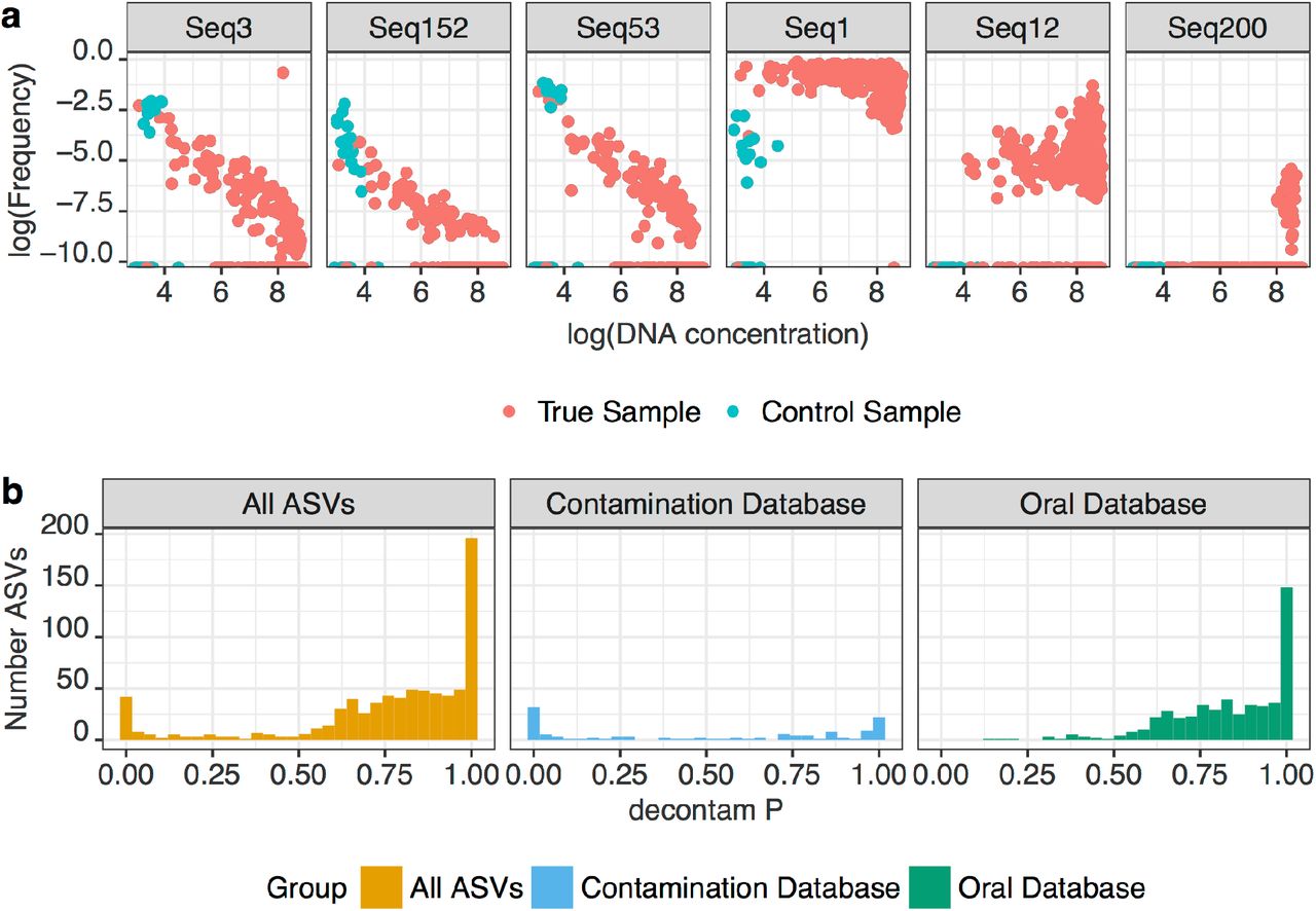
(a) Frequency patterns of six sequences from a 16S rRNA gene study of human oral microbial communities. The frequencies of sequence variants Seq3, Seq152, and Seq53 vary inversely with sample DNA, a characteristic of contaminants. The frequencies of Seq1, Seq12, and Seq200 are independent of sample DNA concentration, a characteristic of sampled taxa. (b) Probabilities for amplicon sequence variants (ASVs) were computed by the “combined” method of the isContaminant function in the decontam R package for all ASVs present in two or more samples (orange), ASVs from genera previously observed as contaminants in negative control samples (blue, Methods) and ASVs from genera known to be members of human oral samples (green, Methods).
decontam discriminates likely contaminating sequences from likely oral sequences
We applied the isContaminant function to all ASVs present in two or more samples in our oral mucosa dataset, selecting the “combined” method which makes use of both frequency and prevalence approaches. The resulting probability distribution was bimodal, with peaks near 0 and 1 (Fig. 2b). Most ASVs (Fig. 2b) and an even larger majority of total reads (Fig. S2) were assigned high probabilities.
To assess the classification accuracy of decontam, we generated two databases to serve as proxies for oral sequences and contaminants (Methods). The oral database contained microbial genera that have been visualized by microscopy in human oral plaque samples. The contamination database contained genera previously sequenced from negative control samples in 16S rRNA gene studies. Most ASVs from genera present in the contamination database were assigned probabilities less than 0.5, while most ASVs from genera present in the oral database were assigned probabilities greater than 0.5 (Fig. 2b). These probability differences were more pronounced when accounting for ASV abundances (Fig. S2). These patterns suggest that decontam effectively differentiated contaminants from genera likely to be members of the oral microbiota.
Thirty-three ASVs in the contamination database had probabilities greater than 0.9, indicating that their frequency and prevalence patterns across samples did not provide evidence of contaminant origin. On closer inspection, these 33 putative contaminants belonged to genera that did not appear in our oral database because they have not been visualized in oral plaque samples (Table S1; Methods), but are frequently sequenced from the oral microbiota (Bik et al. 2010, Chen et al. 2011, Eren et al. 2014). This ambiguity illustrates a fundamental limitation of blacklist methods: the removal of taxa previously identified as contaminants can also remove true members of the microbial communities in which those taxa naturally occur.
Application of decontam to a dilution-series test dataset
Our lack of a priori knowledge of the true microbial composition of the oral samples limits the ways we can evaluate the performance of decontam. An alternative approach is to test decontam on samples of known microbial composition. Salter et al. generated a 10-fold dilution series extending over five decades from a high-biomass monoculture of Salmonella bongori. Aliquots from this dilution series were characterized by 16S rRNA gene sequencing performed at three different sequencing centers, and by shotgun sequencing using four different DNA extraction kits (one of which yielded very little DNA and is excluded here). Standard DNA quantitation data were not reported, so the reported 16S qPCR results (Fig. 2 from Salter et al. 2014) were used as a proxy for the DNA concentration of each dilution sample. We assume that all non-S. bongori sequences represent some form of contamination.
The fraction of non-S. bongori sequencing reads classified as contaminants by the frequency method increased as the classification threshold was made less stringent: Over 50% of the putative contaminant amplicon reads and over 80% of the putative contaminant shotgun reads were identified as contaminants at the default threshold P*=0.1 (Fig. 3). Because the sensitivity of our statistical testing approach is lower for sequence features that appear in only a small number of samples, a much smaller fraction of the unique sequence features (i.e. ASVs in the 16S rRNA gene data and genera in the shotgun data) were identified as contaminants. Identifying contaminants on a per-batch basis was more effective than pooling data across the different sequencing centers and DNA extraction kits, which are expected to have different contaminant spectra (Fig. 3).
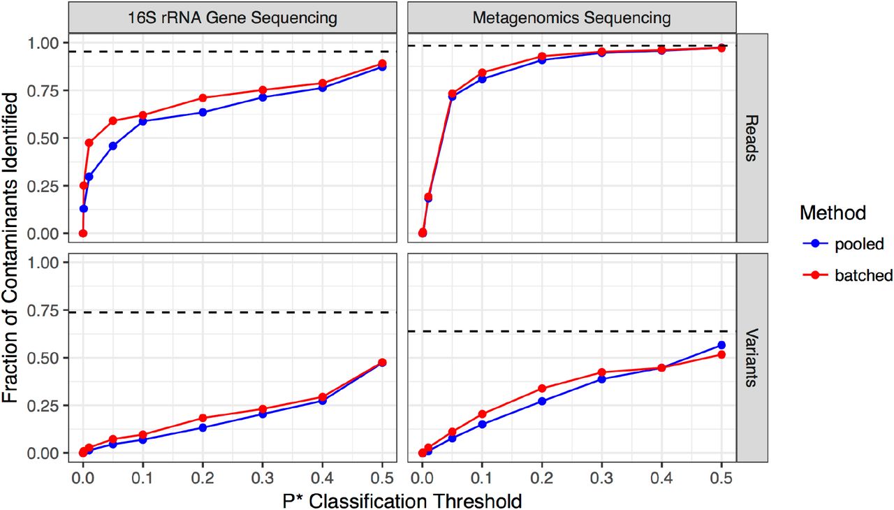
The frequency method was applied to all data pooled together (blue), and on a per-batch basis (red). Batches were specified as the sequencing centers for the 16S data, and the DNA extraction kits for the shotgun data. The fraction of contaminants identified is evaluated on a per-read basis and on a per-variant basis (ASVs for 16S data, genera for shotgun data). Dashed lines show the maximum possible classifier performance, given that decontam cannot identify contaminants only present in a single sample.
Removal of contaminants that were identified by decontam significantly reduced batch effects between samples processed by different sequencing centers and DNA extraction kits (Fig. 4). As the classification threshold increased from P*=0.0 (no contaminants removed) to P*=0.1 (default) to P*=0.5 (aggressive removal), the multi-dimensional scaling ordination distance between samples from different batches decreased. This effect was most dramatic at the intermediate dilutions where both S. bongori and various contaminants made up a significant fraction of the total sequenced DNA, and where decontam almost completely eliminated the separation of samples by batch in the ordination. No S. bongori sequences were removed by decontam: the probabilities of the S. bongori genus and associated ASVs were all > 0.9, well above even the aggressive P*=0.5 classification threshold.

Multi-dimensional-scaling (MDS) ordination of sequenced samples of a monoculture of S. bongori, as a function of dilution and the contaminant classification threshold. A dilution series of 0, 1, 2, 3, 4, and 5 ten-fold dilutions of a pure culture of Salmonella bongori was subjected to 16S rRNA gene sequencing at three sequencing centers, and shotgun sequencing using three different DNA extraction kits. Contaminants were identified by the decontam frequency method with a classification threshold of P*=0.0 (no contaminants identified), P*=0.1 (default), and P*=0.5 (aggressive identification). After contaminant removal, pairwise between-sample Bray-Curtis dissimilarities were calculated, and an MDS ordination was performed. The two dimensions explaining the greatest variation in the data are shown.
The 16S rRNA gene sequencing (but not the shotgun sequencing) data included a negative control from each sequencing center. To test if contaminant classification could be improved by the “prevalence” approach, we grouped the negative control with the two most extreme dilutions to serve as a set of three negative controls (the S. bongori culture was diluted to near absence in dilutions 4 and 5). The “prevalence” approach allowed additional contaminants to be identified (Fig. S1), suggesting that combining the frequency and prevalence approaches is likely optimal when both DNA quantitation data and negative control samples are available.
Identification of non-contaminant sequences in a low-biomass environment
In very low biomass environments, a majority of the sequence features in MGS data might derive from contaminants rather than sequences truly present in the sampled environment. In such cases, it is preferable to require that sequence features show sufficient statistical evidence that they are not contaminants prior to downstream analysis. This alternative approach is naturally supported by switching the null and alternative hypotheses in the “prevalence” approach, and is implemented as the isNotContaminant method in the decontam R package.
Recently it was proposed that the human placenta is not normally sterile but instead harbors an indigenous microbiota, based largely on evidence from marker-gene sequencing of placental samples (Aagard et al. 2014). However, contamination has since been proposed as an alternative explanation of those experimental results (Lauder et al. 2016, Perez-Muñoz et al. 2017). To examine this question further, Lauder et al. performed 16S rRNA gene amplification and sequencing on placenta biopsy samples, as well as a number of negative control samples, using two different DNA extraction kits. Strikingly, samples clustered together by kit rather than by placental or negative control origin, suggesting that most sequences observed in the placenta samples derived from reagent contamination rather than a placenta microbiome.
We applied the isNotContaminant method to the data from Lauder et al. in an effort to determine if any ASVs in their data were consistent with placental origin, despite being too rare to drive whole-community ordination results. Of 557 ASVs present in at least 5 samples, there were 7 ASVs in which the contaminant model was rejected in favor of the non-contaminant model at an FDR threshold of 0.5 (Table 1). However, closer inspection of these ASVs largely rules out the proposed placenta microbiome as a likely source. Five of the 7 ASVs match Homo sapiens, and likely arose from off-target amplification of human DNA present in the placenta biopsy. One of the two putative non-contaminant bacterial ASVs is plausibly explained by translocation during delivery, as it was an exact match to the Lactobacillus crispatus ASV that was the most abundant ASV in the study as a whole and present in every vaginal sample. The other putative non-contaminant bacterial ASV was a Ruminococcaceae variant, a known member of human gut microbial communities (Eckburg et al. 2005).
All 557 ASVs were tested using the isNotContaminant function, with 7 ASVs classified as non-contaminants using an FDR threshold of 0.5 (Benjamini & Hochberg). Taxonomy was assigned by BLAST-ing sequences against the nt database. Prevalence is reported for each sample type.
Reduction of false-positive associations between the maternal microbiota and preterm birth
In a recent study, the vaginal microbiota in gestations that ended in preterm birth (PTB) was compared to the microbiota in gestations ending in term birth in two racially distinct cohorts of women (Callahan & DiGiulio et al. 2017). Exploratory analysis of the associations between Simple statistical identification and removal of contaminant sequences in marker-gene and metagenomics data increased gestational abundances of various bacterial taxa and PTB identified a number of genera associated with PTB (FDR < 0.1 threshold). However, the authors concluded that many of these statistically significant associations were caused by run-specific contaminants rather than a true biological signal.
We applied the isContaminant method to all ASVs in the Callahan & DiGiulio et al. dataset, selecting the “combined” method and specifying the sequencing runs as batches. We then generated a plot similar to the exploratory analysis presented in that paper, but in this case coloring ASVs based on the probabilities determined by isContaminant (Fig. 5). Four of the ASVs most significantly associated with PTB were assigned probabilities less than 10-6, strongly supporting a contaminant origin. The genera to which these ASVs belong are indicated in the figure, and correspond to genera previously observed as contaminants (Herbaspirillum: Barton et al. 2006, Salter et al. 2014, Glassing et al. 2016; Pseudomonas: Salter et al. 2016, Jousselin et al. 2015, Lazarevic et al. 2016, Jervis-Bardy et al. 2015, Glassing et al. 2016; Tumebacillus: Glassing et al. 2016, Kim & Hofstaedter et al. 2017; Yersinia: Afshinnekoo et al. 2015). Removing likely contaminants reduced reported false-positive associations, and improved the power of the exploratory analysis to detect significant associations in the non-contaminant ASVs by reducing the multiple-hypothesis burden.

(A) The association between PTB and an increase in the average gestational frequency of various ASVs was evaluated in the two cohorts of women (Stanford and UAB) analyzed in Callahan & DiGiulio et al. The x- and y-axes display the P values of the association between increased gestational frequency and PTB (one-sided Wilcoxon rank-sum test) in the Stanford and UAB cohorts, respectively. Points are colored by the probability assigned to them by the isContaminant function in the decontam R package, using the combined method. Several ASVs that are strongly associated with PTB in either the Stanford or UAB cohorts are clearly identified as contaminants with a decontam P value of less than 10-5 (genera in magenta text).
Discussion
Previous studies established two common signatures of microbial contaminants in environmental samples: frequency that is inversely proportional to sample DNA concentration (Willner et al. 2012, Lusk 2014, Salter et al. 2014, Jervis-Bardy et al. 2015), and presence in negative control samples (Dunn et al. 2013, Adams et al. 2015, Lazarevic et al. 2016). Building on that work, we developed a simple model of the mixture between contaminating and sample DNA that serves as the basis of a statistical classification method for identifying contaminants in MGS data. This method is implemented in the open source R software package decontam, and can be used to diagnose, identify and remove contaminants in marker-gene and metagenomic sequencing datasets.
We evaluated the accuracy of decontam in a 16S rRNA gene survey of the human oral mucosa, and found that classification of contaminants by decontam largely agreed with literature expectations for contaminant and oral bacterial genera. Furthermore, decontam identified most known contaminant reads in marker-gene and metagenomics datasets generated from a dilution series of a single-species monoculture. Contaminant removal by decontam also improved common downstream analyses. When applied to samples of known composition, decontam reduced technical variation due to sequencing center and DNA extraction kit, an oft-cited issue in high-throughput 16S rRNA gene survey studies (Kennedy et al. 2014, Salter et al. 2014, Sinha et al. 2015). decontam also removed several contaminant taxa from a recent study that a naïve exploratory analysis would have found to be significantly associated with preterm birth (Callahan & DiGiulio et al. 2017). Finally, decontam corroborated another recent study’s conclusion that there was little evidence for a core placenta microbiome in their sequencing data, and extended that conclusion to rare sequences in their dataset (Lauder et al. 2016).
decontam makes significant improvements in current approaches to contaminant identification and removal. First, decontam identifies contaminants on a per-sequence-feature basis, an approach that is lacking from existing software tools. Second, the statistical classification approach employed by decontam avoids several shortcomings of common approaches based on ad hoc thresholds. Removal of all sequences detected in negative controls removes abundant true sequences in the presence of cross-contamination among samples (Wright & Vetsigian, 2016, Edgar 2016). Removal of sequences below an abundance-based cutoff sacrifices low-frequency true sequences, and fails to remove abundant contaminants that are the most likely to interfere with downstream analysis. Together these properties make decontam a useful tool for improving the quality of MGS data, with positive implications for a wide variety of subsequent analyses.
Using decontam
Experimental design
decontam can be used on any dataset in which DNA quantitation data or sequenced negative control samples are available. However, simple experimental design choices can further improve the performance of decontam. Because reagents contribute significantly to contamination (Lusk 2014, Salter et al. 2014, Jervis-Bardy et al. 2015, Lauder et al. 2016), negative control samples containing only reagents or sterile sample collection instruments should be processed and sequenced alongside true biological samples. This will enable use of prevalence-based contaminant identification, which can improve the accuracy of contaminant identification based on frequency alone. Furthermore, because the sensitivity of prevalence-based statistical classification is limited by the number of negative control samples, and because there is often variation between the contaminants observed in different negative control samples, we recommend sequencing multiple negative control samples. Inclusion of a positive control dilution series of samples that covers a broad range of input DNA concentrations may also improve frequency-based contaminant identification (Salter et al. 2014).
Method choice
decontam implements distinct frequency-based or prevalence-based methods for contaminant identification, and can also be instructed to use both methods in combination. Choice of contaminant identification method will be guided first by the availability of the necessary auxiliary data: frequency-based identification requires DNA quantitation data, and prevalence-based identification requires sequenced negative controls.
Effective frequency-based contaminant identification requires variation in sample DNA concentration. We recommend that DNA concentrations vary over at least a two-fold range. In our experience, sufficient variation in DNA concentration typically arises naturally during sample preparation and processing. The inclusion of a dilution series of a positive control sample, as described in Salter et al. 2014, can guarantee a broad range of sample DNA concentrations and may improve the accuracy of frequency-based identification.
The sensitivity of prevalence-based contaminant identification is constrained by the number of sequenced negative control samples, and will have limited power to detect contaminants if few negative control samples are included in the data. In MGS data from very low biomass environments, where contaminant DNA may constitute a large fraction of sequencing reads, the frequency-based identification is not valid and the prevalence-based method implemented in the isNotContaminant function is the best choice.
In our analysis of data from Salter et al., we found that combining the frequency and prevalence approaches was more effective than either method alone. Thus, when both negative controls and DNA quantitation data are available, we recommend using a combination of both methods to identify contaminants. decontam provides multiple ways to combine probabilities from the frequency and prevalence methods into a composite probability that can then be used for classification.
Choice of classification threshold
Sequence features are classified as contaminants by comparing the tail probabilities generated by the selected contaminant identification method to a classification threshold P*. The default value of P*=0.1 separated most expected contaminants from expected oral sequences in our human oral mucosa dataset (100s of samples). In both the oral dataset and in the dilution series from Salter et al. (batches of 6 samples), relaxing the threshold to 0.5 identified additional contaminants with little increase in false positives. Meanwhile, in the pregnancy datasets (1000s of samples), likely false-positive contaminant identifications arose at the default threshold of 0.1, and a more appropriate classification threshold was 0.01 to 0.001.
We recommend that users consider non-default classification thresholds, especially when decontam is being applied in batch-wise fashion such as in large studies that span multiple sequencing runs. Visualization of the probabilities that will be used for classification can identify an appropriate classification threshold. For example, the histogram of probabilities in Figure 2 showed clear bimodality between very low and high probabilities, indicating that classification thresholds in the range from 0.1 to 0.5 would be effective. A second useful visualization is a quantile-quantile plot of probabilities versus a uniform distribution (the “expected” probability distribution).
An alternative way to use the probabilities generated by decontam is as quantitative post-hoc diagnostics, rather than as input to a binary classifier. As suggested by Figure 5, consider a case in which several taxa are identified as differentially expressed in a condition of interest. Inspection of the decontam probabilities associated with those taxa will reveal whether there is statistical evidence that they might have arisen from contaminants, informing subsequent interpretation and speaking to the necessity of further analyses to confirm the validity of those associations.
Application to heterogeneous samples
decontam uses patterns across samples to identify contaminants, but that approach can be less effective when different groups of samples have systematically different contaminant patterns. One such scenario is groups of samples that were processed separately, resulting in different contaminants being introduced in each group. decontam allows the user to specify such “batches” in the data, in which case statistical testing is performed independently within each batch and the most extreme probability across batches is used for contaminant classification. Specification of batches is applicable to studies that span multiple sequencing runs, and should also be considered when other sample processing steps that could introduce contaminants – e.g. differences in DNA extraction kit – differ between groups of samples.
The assumptions of decontam, especially the frequency approach, can also be violated if the methods are applied to groups of samples in which bacterial biomass systematically differs. If, for example, decontam is applied to a set of samples including both stool samples (high biomass) and airway samples (low biomass), the method might flag real sequences that appear in the airway samples as contaminants, because they appear in a higher frequency in the low-concentration samples. Therefore, we recommend applying decontam independently to groups of samples collected from different environments.
Choice of Sequence Feature
decontam can be applied to a variety of sequence features derived from MGS data (e.g. OTUs, ASVs, MAGs). decontam should work most effectively on sequence features that are sufficiently resolved such that they do not group contaminants with real strains, while also not being overly affected by noise arising from MGS sequencing.
In marker-gene data, we expect the best performance will be achieved by using post-denoising ASVs as sequence features, as ASVs separate sequence variants to the maximum extent possible and thus are least prone to grouping contaminants with related real strains. A general recommendation for metagenomics studies is to use finer taxonomic groups (e.g. species rather than families) and narrower functional categories (e.g. genes rather than pathways).
Limitations of decontam and Complementary Approaches
decontam assumes that contaminants and true community members are distinct from one another. This basic assumption fails in the case of cross-contamination, in which sequences from one sample are detected in other samples (Wright & Vetsigian 2016, Edgar 2016). The amount of cross-contamination appears to vary significantly from study to study in ways that are not entirely understood. decontam is not designed to remove cross-contamination, and MGS studies would benefit from new methods to address cross-contamination. We note a recent promising observation that “cross-talk” on Illumina sequences is associated with lower quality index reads, suggesting a simple filtering method to reduce this problem (Wright & Vetsigian 2016).
decontam depends on patterns across samples to identify contaminants, and therefore has low sensitivity for detecting contaminants that are found in few samples. Since very low-prevalence sequences are often uninformative in downstream analyses, it might often be appropriate to combine decontam with a minimum prevalence threshold that removes low-prevalence contaminants that decontam fails to detect. Prevalence thresholds can be applied before or after use of decontam.
Conclusions
Contaminant removal is a critical but often overlooked step in marker-gene and metagenomics (MGS) quality control (Goodrich et al. 2014, Salter et al. 2014, Sinha et al. 2015, Lauder et al. 2016, Kim & Hofstaedter et al. 2017). Salter et al. and Kim & Hofstaedter et al. provide excellent pre-sequencing recommendations that reduce the impact of contamination, which can be complemented by the incorporation of subsequent in silico contaminant removal. Here we introduce a simple, flexible, open-source R package – decontam – that recognizes widely reproduced signatures of contaminant DNA sequences, and guides users in the elimination of these sequences from MGS datasets. decontam is well suited for integrating in silico contaminant removal into the MGS process: it requires only data that are in most cases already generated during sample preparation, readily fits into existing MGS analysis pipelines, and can be applied to many types of MGS data. Together, our results suggest that decontam can improve the accuracy of biological inferences across a wide variety of MGS studies.
Methods
Oral specimen processing
Following extraction of whole genomic DNA using the PowerSoil®-HTP 96 well Soil DNA Isolation Kit (MO BIO Laboratories, Carlsbad, CA, USA), specimens were PCR amplified in 2-4 replicate 75-μL reactions using Golay error-correcting barcoded primers targeting the V4 hypervariable region of the bacterial 16S rRNA gene (Walters et al. 2015). Amplicons were purified, DNA-quantitated using the PicoGreen fluorescence-based Quant-iT dsDNA Assay Kit (ThermoFisher catalog no. Q33120), and pooled in equimolar amounts. Following ethanol precipitation and size-selection, the amplicon pool was sequenced in duplicate on two lanes of an Illumina MiSeq v3 flowcell at the W.M. Keck Center for Comparative Functional Genomics (University of Illinois, Urbana-Champaign, USA).
16S rRNA Gene Sequence Processing
Files from duplicate sequencing runs were concatenated, demultiplexed using Qiime’s split_libraries_fastq.py script, and imported into R for quality filtering, inference of sample composition, and sequence table preparation with the dada2 package (Callahan et al. 2016). The final sequence table consisted of 18,285,750 sequencing reads in 2,420 unique ASVs across 767 samples. Taxonomy was assigned to each sequence using the non-redundant SILVA taxonomic training set (‘silva_nr_v123_train_set.fa’, https://www.arb-silva.de). Auxiliary taxonomy assignment was performed for comparisons of our dataset and past reports of contaminating 16S rRNA gene sequences (see Generation of Recommended Taxonomic Classification).
Construction of Feature Table
The ASV table, taxonomy table, and sample metadata were imported into the phyloseq R package (McMurdie & Holmes, 2013). Samples and taxa were conservatively filtered to include only samples extracted using the same DNA extraction kit, and to remove singleton sequences and ASVs that appeared in only one sample.
Generation of Recommended Taxonomic Classification
To improve taxonomic classification accuracy for oral genera, we classified sequences a second time using the Human Oral Microbiome Database (HOMD, Chen et al. 2011, http://www.homd.org/, ‘HOMD_16S_rRNA_RefSeq_V14.5.fasta’). We then compared SILVA and HOMD classifications at the genus level. For each of 80 sequences on which SILVA and HOMD disagreed, we assigned a recommended genus that best matched genus-level classifications generated by NCBI BLAST.
Construction of oral and contamination databases
To compare our data to past reports of oral microbes and contaminants, we generated two databases. The first contains confirmed members of the human oral microbiota as evidenced by microscopic visualization in human oral specimens (Brinig et al. 2003, Valm et al. 2011, Mark Welch et al. 2016). These microbial genera are listed with their literature citations in the ‘oral_database.csv’ file. A second database captured bacterial genera previously reported as contaminants in 16S rRNA gene negative control samples. The list of genera with their literature citations can be found in the ‘contamination_database.csv’ file. Genera that appeared in both databases were excluded from the contamination database to prevent abundant oral genera that have also been observed as contaminants, like Haemophilus and Streptococcus, from dominating analyses of our data. Note that, although a database derived from oral plaque taxa serves as a reasonable proxy for membership in the oral mucosa, and should exclude contaminants derived from non-oral sites, oral microbes are tissue- and site-specific. Thus, our database may lack a subset of mucosal taxa.
Construction of oral and contamination databases
The sequencing data from the human oral microbiome are available at the SRA under accession number: Pending. The R markdown analysis scripts and all input data necessary to reproduce the analyses in this paper are available at https://benjjneb.github.io/DecontamManuscript/
Acknowledgments
We thank the study participants for specimen donation, and Dr. Ava Wu and Danielle Drury at the UCSF School of Dentistry for collecting oral mucosa specimens. We thank Les Dethlefsen and members of the Relman Lab for helpful discussions and suggestions. This research was supported by NIH National Institute of Dental and Craniofacial Research grant R01 DE023113 (to D.A.R.) and the Thomas C. and Joan M. Merigan Endowment at Stanford University (D.A.R.).
References


