

Abstract
The structure and function of the gut microbiome are shaped by a combination of ecological and evolutionary forces. While the ecological dynamics of the community have been extensively studied, much less is known about how strains of gut bacteria evolve over time. Here we show that with a model-based analysis of existing shotgun metagenomic data, we can gain new insights into the evolutionary dynamics of gut bacteria within and across hosts. We find that long-term evolution across hosts is consistent with quasi-sexual evolution and purifying selection, with relatively weak geographic structure in many prevalent species. However, our quantitative approach also reveals new between-host genealogical signatures that cannot be explained by standard population genetic models. By comparing samples from the same host over ~6 month timescales, we find that within-host differences rarely arise from the invasion of strains as distantly related as those in other hosts. Instead, we more commonly observe a small number of evolutionary changes in resident strains, in which nucleotide variants or gene gains or losses rapidly sweep to high frequency within a host. By comparing the signatures of these mutations with the typical between-host differences, we find evidence that many sweeps are driven by introgression from existing species or strains, rather than by de novo mutations. These data suggest that bacteria in the microbiome can evolve on human relevant timescales, and highlight the feedback between these short-term changes and the longer-term evolution across hosts.
INTRODUCTION
The gut microbiome is a complex ecosystem comprised of a diverse array of microbial organisms. The abundances of different species and strains can vary dramatically based on diet (1), host-species (2), and the identities of other co-colonizing taxa (3). These rapid shifts in community composition suggest that individual gut microbes may be adapted to specific environmental conditions, with strong selection pressures between competing species or strains. Yet while these ecological responses have been extensively studied, much less is known about the evolutionary forces that operate within populations of gut bacteria, both inside individual hosts, and across the larger host-associated population. This makes it difficult to predict how rapidly strains of gut microbes will evolve new ecological preferences and traits when faced with environmental challenges, and how the genetic fingerprint of the community will change as a result.
The answers to these questions depend on two different types of information. At a mechanistic level, we must understand the functional traits that are under selection in the gut, and the range of genetic mutations that can alter these traits. Although it can be challenging to measure such selection pressures in vivo, comparative genomics (4, 5), experiments in model organisms (6, 7), and high-throughput screens (8, 9) are starting to provide valuable information about the functional traits required to thrive in the gut environment.
In addition to this raw material, we must also understand the population genetic processes that govern how mutations spread through a population of gut bacteria, both within individual hosts, and across the larger population. But in contrast to well-studied examples in pathogens (10), laboratory evolution experiments (11), and some environmental communities (12, 13, 14, 15), much less is known about the population genetic processes that operate within species of commensal gut bacteria. In the well-studied examples above, previous work has shown that evolutionary dynamics are often dominated by rapid adaptation, with new variants accumulating within months or years (6, 12, 16, 17, 18, 19, 20, 21, 22, 23). Theory predicts that such rapid evolutionary dynamics can strongly influence which mutations are able to fix within a population (24, 25), and the amount of genetic diversity that these populations can maintain (26, 27).
However, it is not clear how this existing picture of microbial evolution extends to a more complex and established ecosystem like the healthy gut microbiome. On the one hand, hominid gut bacteria have had many generations to adapt to their host environment (28), and may not be subject to the continually changing immune pressures faced by many pathogens. The large number of potential competitors in the gut ecosystem may also provide fewer opportunities for a strain to adapt to new conditions before an existing strain expands to fill the niche (29, 30) or a new strain invades from outside the host. On the other hand, small-scale environmental fluctuations, either driven directly by the host or through interactions with other resident strains, might increase the opportunities for local adaptation (31). If immigration is restricted, the large census population size of gut bacteria could allow residents to produce and fix adaptive variants rapidly before a new strain is able to invade. In this case, one might expect to observe rapid adaptation on short timescales, which is eventually arrested on longer timescales as strains are exposed to the full range of host environments. Determining which of these scenarios apply to gut communities is critical for efforts to study and manipulate the microbiome.
Amplicon sequencing provides limited resolution to distinguish between these competing models of microbiome evolution (32). But, with the increasing availability of whole-genome metagenomic samples, particularly from human hosts, we now have the raw polymorphism data necessary to address such evolutionary questions (33).
However, there is still a technical challenge: it is difficult to resolve evolutionary changes between specific lineages using pooled short-read sequencing of a complex microbial community. As a result, previous studies have largely focused on the overall differences in genetic diversity between samples (33, 34, 35, 36, 37), rather than the differences in their constituent lineages. While sophisticated algorithms for strain detection have been developed (38, 39, 40), this remains a difficult problem, and it is likely that new sequencing (41, 42) or culturing (43) techniques will be required to fully resolve human microbiome haplotypes. In this study, we take a different approach to the strain detection problem, which leverages the large number of high-coverage human gut metagenomes currently available. Building on earlier work (4, 40), we show that in many prevalent species, there are a subset of hosts with particularly simple lineage structures where the dominant haplotype is easier to identify. By focusing on these “confidently phaseable” samples, we develop methods for resolving evolutionary changes between the dominant lineages with a high degree of confidence.
We use this approach to analyze a large panel of publicly available human stool samples (44, 45, 46), to quantify the population genetic forces (e.g. selection, recombination, and drift) that operate within and across hosts. Across hosts, we find that the long-term evolutionary dynamics are broadly consistent with models of quasi-sexual evolution and purifying selection, with relatively weak geographic structure in many prevalent species. However, our quantitative approach also reveals interesting departures from standard population genetic models. Given the large sample sizes involved (many sequenced metagenomes, each with multiple resident species), these results suggest that the microbiome may be a useful system for studying general features of microbial population genetics that apply across many species.
We also use our approach to detect examples of within-host adaptation, in which nucleotide variants or gene gain or loss events rapidly sweep to high frequency within the ~ 6 month sampling window. Furthermore, we find evidence that many of these within-host sweeps are driven by introgression from existing species or strains, rather than by de novo mutations, consistent with the theory that there are many such routes for adaptation in a complex ecosystem with large census population sizes and frequent horizontal exchange. Together, these data suggest a preliminary model of evolution in the gut microbiome, which can be refined as more sophisticated sequencing technologies and longitudinal studies become more common.
RESULTS
DATA AND VARIANT CALLING
We analyzed whole-genome sequence data from a panel of 499 stool samples taken from 365 healthy human subjects (Table S1). 314 of these samples were sequenced by the Human Microbiome Project (44), and were taken from 180 individuals from two U.S. cities. 52 of these individuals were sampled at two timepoints roughly 6 months apart and 41 individuals were sampled at three timepoints over the span of ~ 1 year. We used these longitudinal samples to study within-host changes on short timescales. To control for geographic structure, we also included samples from a Chinese cohort (185 individuals sampled once) with similar sequencing characteristics (45).
We analyzed these data using a reference-based approach that leverages the MIDAS pipeline (47) (SI Section 1). Briefly, sequencing reads were aligned to a panel of reference genomes, which were chosen to represent different bacterial "species" based on sequence identity. Putative single-nucleotide variants (SNVs) within each species were determined from the pileup of reads at a given site. Stringent quality, alignment, depth, and breadth thresholds were chosen to reduce mapping artifacts (see SI Section 1). For similar reasons, we only considered SNVs in annotated coding regions on the reference genome.
To quantify variation in gene content, sequencing reads were also aligned to a panel of pangenomes, constructed by pooling genes from sequenced isolates for each bacterial species. The relative coverage of genes was used to quantify gene content variation and to define a “core genome” for each species, defined as the set of genes present in the reference genome and in ≥ 90% of the samples in our panel. All other genes were defined to be “accessory” genes. We used these annotations to analyze certain subsets of the SNVs detected on the reference genome, as indicated below.
RESOLVING WITHIN-HOST LINEAGE STRUCTURE
To investigate the population genetic forces in the gut microbiome, we wish to identify mutations that accumulate along different lineages within a given species. However, we cannot directly observe these lineages in shotgun metagenomic data, since the primary observations are allele frequency estimates from a mixed-population sample. To measure genetic changes between lineages, we must first understand the lineage structure that is present in individual hosts, so that we may later associate allele frequencies with mutations on specific lineages.
Several previous studies have investigated within-species diversity in human gut metagenomes (33, 36, 40, 47). These studies have found that (i) metagenomes from different hosts harbor many fixed differences between them, (ii) species differ in the average amount of polymorphism that is present within hosts, and (iii) hosts also vary widely in the amount of polymorphism that is present for a given species. Here, we show how these patterns emerge from the lineage structure that is set by the host colonization process, and how certain aspects of this lineage structure can be inferred from the statistics of within-host polymorphism.
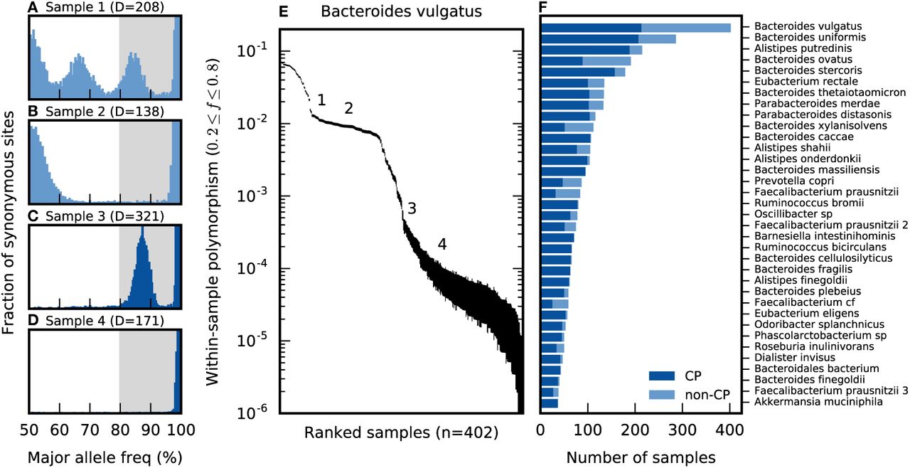
As an illustrative example, we first focus on the patterns of polymorphism in Bacteroides vulgatus, which is among the most abundant and prevalent species in the human gut. This ensures that the B. vulgatus genome has high-coverage in many samples, which enables more precise estimates of the allele frequencies in each sample (Fig. 1A-D). The overall levels of within-host diversity for this species are summarized in Fig. 1E, based on the fraction of synonymous sites in core genes with intermediate allele frequencies (0.2 ≤ f ≤ 0.8, i.e. major allele frequencies in the white region in Figs. 1A-D). The rate of intermediate- frequency polymorphism varies widely among the samples: some metagenomes have only a few variants per genome, while others have mutations at more than 1% of all synonymous sites, which is comparable to the differences between samples (Fig. S2).

(a-d) The distribution of major allele frequencies at synonymous sites in the core genome of Bacteroides vulgatus for four different samples, with the median core-genome-wide coverage listed above each panel. The shaded region denotes major allele frequencies greater than 80%, and the vertical axis is truncated for visibility. (e) The average fraction of synonymous sites in the core genome with major allele frequencies ≤ 80%, for different samples of B. vulgatus. Vertical lines denote 95% posterior confidence intervals based on the observed number of counts (SI Section 9). For comparison, the samples in panels (a-d) are indicated by the numbers (1-4). (f) The distribution of confidently phaseable (CP) samples among the 35 most-prevalent species, arranged by descending prevalence; the distribution across hosts is shown in Fig. S4. For comparison, panels (c) and (d) are classified as confidently phaseable, while panels (a) and (b) are not.
The simplest model of within-host polymorphism assumes that each host is colonized by a single bacterial clone, so that the intermediate variants represent mutations that have arisen since colonization. However, this model cannot quantitatively account for the hosts with higher rates of polymorphism in Fig. 1E. Given conservatively high estimates for per site mutation rates [µ ~ 10−9 (48)], generation times [~ 10 per day (49)], and time since colonization [< 100 years], we would expect a neutral polymorphism rate < 10−3 at each synonymous site (SI Section 2). Instead, we conclude that the samples with higher synonymous diversity must have been colonized by multiple bacterial lineages that diverged for many generations before colonizing the host.
A plausible alternative to the single-colonization model would involve a large number of colonizing lineages (nc ≫ 1) drawn at random from the broader population. However, this process is expected to produce fairly consistent polymorphism rates and allele frequency distributions in different samples, which is at odds with the variability we observe even among the high-diversity samples (e.g., Figs. 1A,B). Instead, we hypothesize that many of the high-diversity hosts have been colonized by just a few pre-existing lineages [i.e.,  . Consistent with this hypothesis, the distribution of allele frequencies in each host is often strongly peaked around a few characteristic frequencies (Fig. 1A-D), suggesting a mixture of several distinct lineages. Similar findings have recently been reported in a number of other host-associated microbes, including several species of gut bacteria (4, 40, 50, 51). Figures 1A-C show that hosts can vary both in the apparent number of colonizing lineages, and the frequencies at which they are mixed together. As a result, we cannot exclude the possibility that even the low diversity samples (e.g. Fig. 1D) are colonized by multiple lineages that happen to fall below the detection threshold set by the depth of sequencing. We will refer to this scenario as an “oligo-colonization” model, in order to contrast with the single-colonization (nc = 1) and multiple-colonization (nc ≫ 1) alternatives above.
Confidently phaseable (CP) samples
Compared to the single- and multiple-colonization models, the oligo-colonization model makes it more difficult to identify evolutionary changes between lineages. In this scenario, individual hosts are not clonal, but the within-host allele frequencies derive from idiosyncratic colonization processes, rather than a large random sample from the population. To disentangle genetic changes between lineages from these host-specific factors, we must estimate phased haplotypes from the distribution of allele frequencies within individual hosts. This is a complicated inverse problem (38), and we will not attempt to solve the general case here. Instead, we adopt an approach similar to Truong et al. (40) and others, and leverage the fact that the lineage structure in some hosts is simple enough that we can infer one of the dominant haplotypes with a high degree of confidence.
Our approach is based on the observation that whenever the major alleles at two sites are sufficiently common, an appreciable fraction of cells must possess both major alleles (SI Section 3.1). This theoretical argument suggests that we can phase a portion of one of the haplotypes in a metagenome by taking the major alleles present above some threshold frequency f* ≫ 50%, and treating the remaining sites as missing data.
However, we do not observe the true allele frequency directly, but rather an estimated value from a finite sample of sequencing reads. This can lead to phasing errors when the true major allele is sampled at low frequency by chance, and is therefore assigned to the opposite lineage (Fig. S1). The probability of an error increases as sequencing coverage decreases and as the major allele frequency approaches 50% (SI Section 3.2). Prior approaches based on consensus alleles did not provide explicit expressions for these polarization errors. By modeling the error process, we show that the expected probability of a polarization error (given the coverage thresholds in SI Section 1) can be bounded to be sufficiently low if we take f* = 80%, and if we restrict our attention to samples with sufficiently low rates of intermediate-frequency polymorphism in the species of interest (SI Section 3.3). We will refer to the samples that pass this criteria for a given species as confidently phaseable (CP) samples; in the example above, Figs. 1C,D are classified as confidently phaseable for B. vulgatus, while Figs. 1A,B are not.
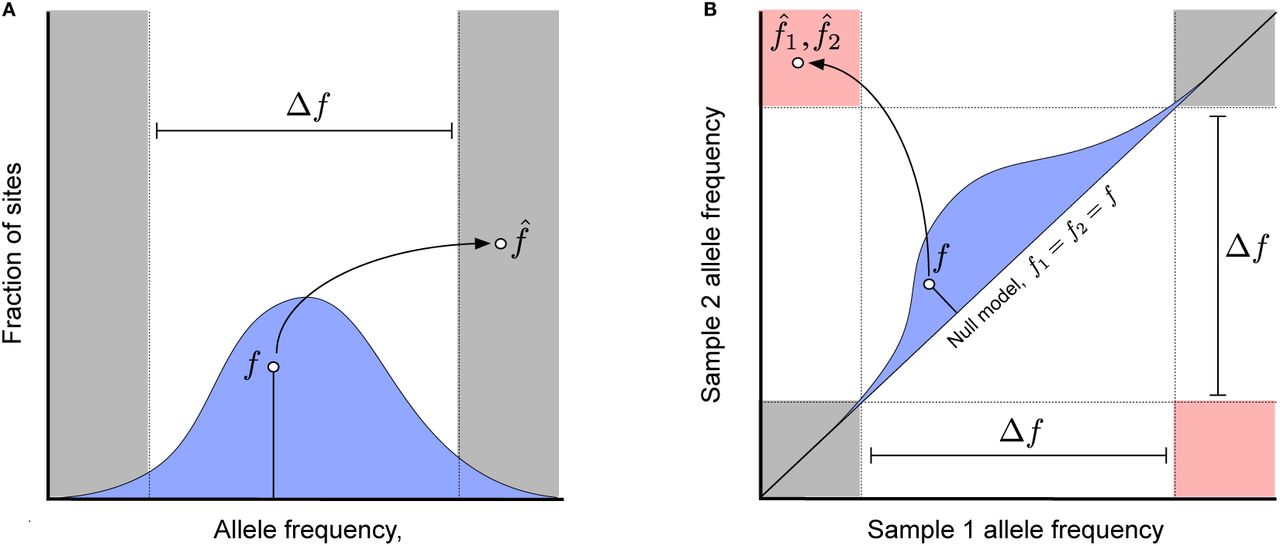
(a) An example of a haplotype phasing error, where an allele with true within-host frequency f [drawn from a hypothetical genome-wide prior distribution, p0(f), blue] is observed with a sample frequency  with the opposite polarization. (b) An example of a falsely detected nucleotide substitution between two samples, where an allele with true frequency f1 = f2 = f [drawn from a hypothetical genome-wide null distribution, p0(f), blue] is observed with a sample frequency
  in one sample and
  in another. Allele frequency pairs that fall in the pink region are counted as nucleotide differences between the two samples, while pairs in the grey shaded region are counted as evidence for no nucleotide difference; all other values are treated as missing data.
In Fig. 1F, we plot the distribution of CP samples across the most prevalent gut bacterial species in our panel. The fraction of CP samples varies between species, ranging from ~ 50% in the case of P. copri to nearly 100% for B. fragilis (4), and it accounts for much of the variation in the average polymorphism rate (Fig. S3). Most individuals carry a mixture of CP and non-CP species (Fig. S4). Thus, while many species-sample combinations lack this simple lineage structure, in a cohort of a few hundred samples it is not uncommon to find ≥ 50 CP samples in many of the most prevalent species. Aggregating across species, we were able to estimate ~ 3000 partially-phased haplotypes from the ~ 500 metagenomic samples in our data set. Among the longitudinally sampled individuals in the HMP cohort, a majority of individuals maintain their CP/non-CP classification at both timepoints (Fig. S5). However, there are still examples of non-CP samples transitioning to CP, and vice versa, so the stability is not universal. We will revisit the peculiar properties of this within-host lineage distribution in the Discussion. For the remainder of the analysis, we will take the distribution in Fig. 1F as given and focus on leveraging the CP samples to quantify the evolutionary changes that accumulate between lineages in different samples.

(a) The fraction of fourfold degenerate synonymous sites in the core genome that have major allele frequencies ≥ 80% and differ in a randomly selected sample (see SI Section 3.3 for a formal definition). (b) The corresponding rate of intermediate-frequency polymorphism for each sample, reproduced from Fig. 1B. In both panels, samples are plotted in the same order as in Fig. 1B.

Symbols denote the average rate of within-host polymorphism (as defined in Fig. 1E) for each species as a function of the fraction of non-CP samples in that species.

Left: The distribution of the fraction of CP species per sample (blue line). The grey line denotes the corresponding null distribution obtained by randomly permuting the CP classifications across the samples. Right: The number of species classified as CP in each sample on the left as a function of the number of species in that sample. A small amount of noise is added to both axes to enhance visibility.

Species are arranged in decreasing order of sample size. Only species with ≥ 5 longitudinally sampled individuals are included.
We investigate two types of changes between lineages in different CP samples. The first class consists of single nucleotide differences, which are defined as SNVs that transition from allele frequencies ≤ 1 − f* in one sample to ≥ f* in another, with f* ≈ 80% as above (Fig. S1). These thresholds are chosen to ensure a low genome-wide false positive rate given the typical coverage and allele frequency distributions among the CP samples in our panel (SI Section 3.4). The second class consists of differences in gene presence or absence, in which the relative copy number of a gene, c, transitions from a value below the threshold of detection (c < 0.05, which is equivalent to < 5% of the coverage of a single-copy gene, or less than five copies per 100 cells) to the range in which the majority of single-copy genes lie (0.5 < c < 2, see Fig. S6). These thresholds are chosen to ensure a low genome-wide false positive rate across the CP samples given the typical variation in sequencing coverage along the genome (SI Section 3.5).

The grey region denotes the copy number range required in at least one sample to detect a difference in gene content between a pair of samples (see SI Section 3.5).
Note that these SNV and gene changes represent only a subset of the potential differences between lineages, since they neglect other evolutionary changes (e.g., indels, genome rearrangements, or changes in high copy number genes) that are more difficult to quantify in a metagenomic sample, as well as more subtle changes in allele frequency and gene copy number that do not reach our stringent detection thresholds. We will revisit these and other limitations in more detail in the Discussion.
LONG-TERM EVOLUTION ACROSS HOSTS
By focusing on CP samples, we can measure differences between haplotypes in different hosts, as well as within hosts over short time periods. To interpret the within-host changes that we observe, it will be useful to first understand the structure of genetic variation between lineages in different CP hosts. This variation reflects the long-term population genetic forces that operate within each species, integrating over many rounds of colonization, growth, and dispersal.
To investigate these forces, we first analyzed the total nucleotide divergence between the phased lineages from different pairs of CP hosts, for a given bacterial species. B. vulgatus will again serve as a useful case study, since it has the largest number of CP hosts to analyze. Figure 2A shows a UPGMA dendrogram of these pairwise distances, averaged across the core genome of B. vulgatus. In a panmictic, neutrally evolving population, we would expect these distances to be clustered around an effective population size for the across-host population, d ≈ 2µNe (52). In contrast, we observe striking differences in the degree of relatedness between the lineages in Fig. 2A. Even at this coarse, core-genome-wide level, the genetic distances vary over several orders of magnitude. Similarly broad ranges of divergence are observed in many other prevalent species as well (Fig. 3A), particularly in the Bacteroides genus. We investigate potential causes of this phenomenon below by focusing on the high and low tails of the divergence distribution.

(a) Dendrogram constructed from the average nucleotide divergence across the core genome of B. vulgatus in different pairs of CP hosts, based on UPGMA clustering (SI Section 4). The underlying distribution of distances and their corresponding uncertainties are shown in Fig. S7. Each host is colored according to its geographic location. Branches with anomalously short divergence rates (d < 2 × 10⁻⁴) are highlighted in bold. (b) The fraction of phylogenetically inconsistent SNPs as a function of divergence (SI Section 4.2). The observed values are shown in red, while the expectations assuming independence between the loci (‘unlinked’ loci) are shown in grey for comparison. (c,d) Analgous versions of (a) and (b) for Bacteroides stercoris.

Nucleotide divergence across the core genome of B. vulgatus for (a) 500 random host pairs, sorted in descending order, and (b) the 100 most closely related pairs, for comparison. For each pair, vertical lines denote 95% posterior confidence intervals based on the observed number of counts (SI Section 9) (c,d). Analogous versions of panels (a) and (b) for B. stercoris.

(a) Distribution of nucleotide divergence at all sites in the core genome between pairs of CP hosts (plotted in grey), across a panel of prevalent species. Species are sorted according to their phylogenetic distances (47), with the number of CP hosts indicated in parentheses; species were only included if they had at least 33 CP hosts (> 500 CP pairs). Symbols denote the median (dash), 1-percentile (small circle), and 0.1-percentile (large circle) of each distribution, and are connected by a red line for visualization; for species with less than 1000 CP pairs, the 0.1-percentile is estimated by the second-lowest divergence value. The dashed line denotes our ad-hoc definition of “closely related” divergence, d ≤ 2 × 10⁻⁴ for a pair of CP hosts. Many species have some pairs of closely related hosts. (b) The distribution of the number of closely related strains per pair of hosts (across species). The null distribution is obtained by randomly permuting hosts independently within each species (n = 1000 permutations, P ≈ 0.9). (c) The cumulative distribution of the number of gene content differences for all pairs in panel A (black), i.e., all choices of species x host 1 x host 2. The red line shows the corresponding distribution for the subset of closely related strains. For comparison, the grey line denotes a ‘clock-like’ null distribution for the closely related strains, which assumes that genes and SNVs each accumulate at constant rates. (d) Ratio of divergence at nondegenerate nonsynonymous sites (dN) and fourfold degenerate synonymous sites (dS) as a function of synonymous divergence for all pairs in panel A (grey circles). Pairs from B. vulgatus are highlighted in red for comparison. Crosses (x) denote species-wide estimates obtained from the ratio of the median dN and dS within each species. The black line denotes the theoretical prediction from the purifying selection null model in SI Section 5. (inset) Ratio between the cumulative dN and dS values for all CP host pairs with core-genome-wide synonymous divergence less than dS. Shaded region denotes ±2 standard deviation confidence intervals estimated by Poisson resampling.
Evidence for subspecies at high divergence rates
At the highest genetic distances in Fig. 2A, the B. vulgatus lineages are partitioned into two deeply-diverged clades, with substantially lower divergence within each clade (Fst ≈ 0.6 between the two clades, Fig. S8). This gap in the divergence distribution (Fig. S7A) suggests that the clades may represent distinct subspecies that both meet the MIDAS sequence similarity threshold for belonging to the B. vulgatus species. Consistent with this hypothesis, the majority of SNVs are specific to one clade or the other, and are rarely shared between clades (Fig. 2B).

Top panel: Fst between manually assigned top-level clades (i.e., groups of deeply diverged lineages in the lineage tree) for each species, as defined in Table S2. Species are only included if there are at least two clades with more than two individuals in each of them. The dashed line denotes the upper range of the middle panel below. Middle panel: Fst between HMP (US) and Chinese samples. Observed values are plotted as symbols, and the null distributions (obtained by randomly permuting country labels) are shown in grey. Significant Fst values (p < 0.05) are indicated with a square symbol. Bottom panel: likelihood ratio statistic assessing whether (manually assigned) clades are better predictors of country of origin. Species are included only if there are at least two clades with more than two individuals. Observed values are plotted as symbols (significant=square, non-significant=circle), while the null distributions (obtained by randomly permuting country labels) are shown in grey.
Furthermore, this clade structure does not appear to be a simple consequence of isolation by distance (or related models like isolation-by-diet). Not only is there no strong correlation between clade and country of origin in Fig. 2A, but there are also non-CP B. vulgatus samples with high within-host polymorphism rates that contain lineages from both clades simultaneously (Fig. 1E). This provides additional evidence that the deeply-diverged clades may be distinct subspecies.
Across the most prevalent species of gut bacteria, we find several other examples of strong (yet geographically uncorrelated) deeply-diverged clades (Fig. S8). But this is not a universal pattern across gut bacteria: some species, even other Bacteroides like Bacteroides stercoris, have lineage phylogenies more consistent with a single clade (Fig. 2C). In a minority of cases [most of which have been previously identified (33, 36, 40)], the deeply-diverged clades are more strongly correlated with geographic location (see SI Section 4.3).
Anomalously low divergence rates
The presence of subspecies at high divergence (> 1%) is not unexpected, since our species boundaries are defined operationally using the sequence similarity of existing reference genomes. A more surprising feature of Figs. 2 and 3 are the many pairs of lineages with extremely low divergence across the core genome (e.g. ≲ 0.01%), more than an order of magnitude below the typical between-host differences. These pairs of lineages are found in many different subclades and appear to be fairly uniformly distributed across the tree for each species (bolded branches in Figs. 2A,C).
Closely related strains can arise naturally in a large sample when two cells are sampled from the same clonal expansion (a breakdown of random sampling). However, such simple explanations are unlikely to apply here. Not only are the lineages sampled from different hosts, but we can also find pairs of closely related strains in Figs. 2A,C from different U.S. cities or different continents. Moreover, pairs of hosts with closely related strains in one species do not typically have closely related strains of other species (Fig. 3B), which allows us to rule out other host-wide sampling biases.
Though the the rates of divergence between these sister lineages are small, they are still significantly larger than the estimated false positive rate (SI Section 3.4), so the core genomes are genetically distinct. In addition, the closely related strains differ substantially in their gene content, with ~ 100 gene differences separating the two lineages (Fig. 3C). This suggests that the closely related strains represent a true intermediate genealogical timescale in bacterial population genetics, whose cause is yet unknown. This hypothesis is bolstered by the large number of prevalent species in Fig. 3A with anomalously low divergence rates. However, this pattern is also not universal: some genera, like Alistipes or Eubacterium, show more uniform rates of divergence between hosts. Apart from these phylogenetic correlations, there are no obvious explanations for the differences between species [e.g., sample size, abundance, vertical transmissibility (47), sporulation score (53)].
Different patterns of natural selection on short timescales
Given the existence of anomalously low divergence rates, we next asked whether natural selection behaves differently for mutations that accumulate on these shorter timescales, compared to the typical divergence rates between lineages. We focused on a common coarse-grained measure of natural selection by comparing the relative contribution of synonymous and nonsynonymous mutations that comprise the overall divergence rates in Fig. 3A. Specifically, we focused on the ratio between the per-site divergence at nonsynonymous sites (dN) and the corresponding value at synonymous sites (dS). Under the assumption that synonymous mutations are effectively neutral, the ratio dN/dS measures the average action of natural selection on mutations at nonsynonymous sites.
In Fig. 3D, we plot the distribution of dN/dS across every pair of CP hosts in each of the prevalent species in Fig. 3A. The values of dN/dS are plotted as a function of dS (a proxy for the average divergence time across the genome). We observe a consistent negative relationship between these two quantities across the prevalent species in Fig. 3.
For large divergence times (dS ~ 1%), the fraction of nonsynonymous mutations is approximately dN/dS ~ 0.1, similar to previously reported values (33), indicating widespread purifying selection. Yet among the closely related strains (dS ~ 0.01%), we observe a much higher fraction of nonsynonymous changes (dN/dS ~ 1). The variation in dN/dS as a function of dS is much more pronounced than the variation between the typical values of dN/dS within each species (black crosses in Fig. 3D). While the latter may be driven by mutational biases, the stronger within-species signal indicates that there are consistent differences in the action of natural selection as a function of time. This provides further support for the hypothesis that anomalously low values of dS arise from a separate genealogical process.
The trend in Fig. 3D is consistent with a simple null model, in which purifying selection is less efficient at purging deleterious variants on shorter timescales (SI Section 5). In particular, we can reproduce the quantitative shape of Fig. 3D with a simple distribution of fitness effects, in which 90% of nonsynonymous variants have fitness costs on the order of s/µ 105, with the remaining sites being neutral. However, while this is the simplest possible null model that can explain the data, we cannot exclude more elaborate explanations for this trend, like enhanced adaptation and hitchhiking on short timescales, or a recent global shift in selection pressures caused by host-specific factors (e.g., the introduction of agriculture).
Quasi-sexual evolution on intermediate timescales
In principle, genome-wide patterns of divergence similar to Figs. 2 and 3 could arise in a model with strong population structure, in which all but the most closely related strains are genetically isolated from each other (54). However, while this model may apply to the most deeply-diverged clades in certain species (e.g. B. vulgatus), we will now show that such genetic isolation does not hold for intermediate divergence times (i.e. below the top level clades in Table S2 but with d ≲ 10−3) that separate typical pairs of strains in different hosts.
Our first line of evidence derives from inconsistencies in the dendrograms in Figs. 2A,C. In both Bacteroides species, a substantial fraction of core-genome SNVs that segregate in intermediate-divergence clades are inconsistent with core-genome- wide dendrogram (i.e., they are also polymorphic outside the clade, see SI Section 4.2). Moreover, the fraction of inconsistent core-genome SNVs is nearly indistinguishable from the expectation under a model of free recombination (Figs. 2B,D). Yet while this phylogenetic inconsistency is suggestive of recombination, it can also arise from purely clonal mechanisms (e.g., recurrent mutation), or from statistical uncertainties in the genome-wide tree.
We therefore sought additional evidence of recombination by examining the decay of linkage disequilibrium (LD) between pairs of synonymous SNVs in the core genome of each species. We quantified linkage disequilibrium using a standard (55) measure of gametic correlation,  , with an unbiased estimator to control for varying sample size (SI Section 6). The overall magnitude of
  depends on various factors (e.g., demography), while changes in
  between different pairs of loci reflect differences in the effective recombination rate (56). By focusing on CP samples, we can estimate
  between SNVs that are separated by more distance (along the reference genome) than a typical sequencing read. However, since the synteny of individual lineages may differ substantially from the reference genome, we only assigned coordinate distances (ℓ) to pairs of SNVs in the same gene, which are more likely (but not guaranteed) to be nearby in the genomes in other samples; all other pairs of SNVs are grouped together in a single category (“core-genome-wide”). We then estimated
  as a function of ℓ for each of these distance categories (SI Section 6), and analyzed the shape of this function.
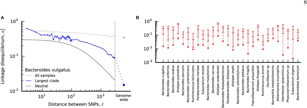
As an example, Fig. 4A illustrates the estimated values of σ2(ℓ) for B. vulgatus; summarized versions of this function are shown for the other prevalent species in Fig. 4B. In almost all cases, we find that core-genome-wide LD is significantly lower than for pairs of SNVs in the same core gene, suggesting that much of the phylogenetic inconsistency in Fig. 2 is caused by recombination. In principle, this intergenic recombination could be driven by the exchange of operons or other large clusters of genes, which often co-segregate in plasmid or transposon vectors in bacteria (57). However, we also observe a significant decay in LD within individual genes (Fig. 4), suggesting a role for more traditional mechanisms of homologous recombination as well.

(a) Linkage disequilibrium  as a function of distance (ℓ) between pairs of fourfold degenerate synonymous sites in the same core gene in B. vulgatus (see SI Section 6). Individual data points are shown for distances < 100bp, while the solid line shows the average in sliding windows of 0.2 log units. The grey line indicates the values obtained without controlling for population structure, while the blue line is restricted to CP hosts in the largest top-level clade (Table S2). The solid black line denotes the neutral prediction from SI Section 6; the two free parameters in this model are
  and ℓ scaling factors, which are shifted to enhance visibility. For comparison, the core-genome-wide estimate for SNVs in different genes is depicted by the dashed line and circle. (b) Summary of linkage disequilibrium for CP hosts in the largest top-level clade (see SI Section 6) for all species with ≥ 10 CP hosts. For each species, the three dashes denote the value of
  for intragenic distances of ℓ = 9, 99, and 2001 bp, respectively, while the core-genome-wide values are depicted by circles. Points belonging to the same species are connected by vertical lines for visualization.
The magnitude of the decay of LD within core genes is somewhat less than has been observed in other bacterial species (14), and only rarely decays to genome-wide levels by the end of a typical gene. Moreover, by visualizing the data on a logarithmic scale, we see that the shape of  is inconsistent with the predictions of the neutral model (Fig. 4A), decaying much more slowly with ℓ than the ~ 1/ℓ dependence expected at large distances (55). Thus, while we can obtain rough estimates of r/µ by fitting the data to a neutral model (Fig. S9), these estimates should be regarded with caution because they vary depending on the length scale on which they are measured (SI Section 6). This suggests that new theoretical models will be required to fully understand the patterns of recombination that we observe.

For each species, the two dashes represent effective values of r/µ estimated from the neutral prediction for the decay of  , using the half-maximum and quarter-maximum decay lengths, respectively (see SI Section 6). The two estimates are connected by a vertical line for visualization.
Gene flow on shorter timescales
Given the evidence for recombination, the existence of closely related lineages in unrelated hosts is even more surprising, since this requires strong correlations between a large number of otherwise independent loci. One potential explanation is that the closely related clades are actually genetically isolated on short genealogical timescales (e.g. due to ecological partitioning), and only acquire their quasi-sexual character on much longer timescales by slowly acquiring DNA from the environment. Consistent with this hypothesis, the fraction of phylogenetically inconsistent core-genome SNVs does decline in clades with lower levels of divergence (Figs. 2B,D), though the expectations from the unlinked model show a similar decline as well. Much of this trend is driven by an increase in SNVs that are private to a single lineage, which cannot be phylogenetically inconsistent. In fact, we observe an excess of private SNVs in lineages with anomalously recent branching (Fig. S10), consistent with increased genetic isolation in the recent past. However, we cannot exclude other mechanisms that would influence the fraction of private SNVs, like increased hitchhiking and Hill-Robertson interference (58) on short-timescales. In addition, it is important to note that a significant fraction of the non-private SNVs are still shared outside the low-divergence clades (Figs. 2B,D), and even the most closely related core genomes have gene repertoires that differ by ~ 100 accessory genes. Thus, while there is some evidence for increased genetic isolation at short timescales, any barriers to gene flow are incomplete.
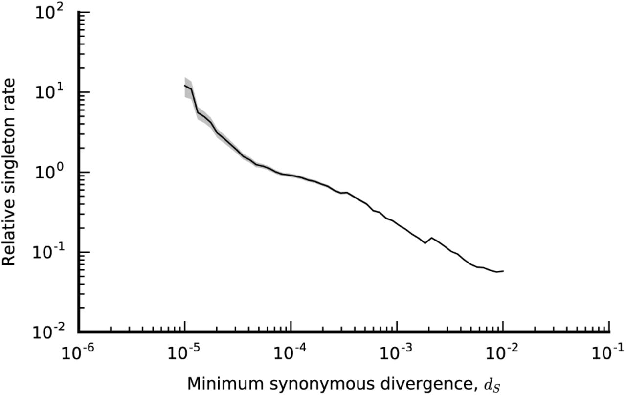
An estimate of the relative singleton rate for all hosts that have core genome synonymous divergence ≤ dS with the next most closely related host. For a given host i, the core genome synonymous divergence with the next closely related host is defined as  , across all other hosts j. For a given value of dS, the relative singleton rate is estimated by dividing the total number of synonymous singleton SNVs across all hosts with
  , by the corresponding number of opportunities, and then by the corresponding total of
  . The shaded region denotes a ±2 standard deviation confidence interval obtained by bootstrap resampling.
SHORT-TERM SUCCESSION WITHIN HOSTS
In the previous sections, we focused on longer-term evolutionary changes that accumulate over many host colonization cycles. However, one of the main advantages of our phasing method is that it can be used to investigate short-term changes within hosts as well. Previous studies of longitudinally sampled metagenomes have shown that on average, two samples from the same host are more similar to each other than to samples from different hosts (33, 40, 46, 47, 59, 60). This suggests that resident sub-populations of bacteria often persist within hosts for ≳ 1 year (~ 300 − 3000 generations), potentially enough time for evolutionary adaptation to occur (6). However, the limited resolution of previous metagenome-wide (33) or species-averaged (40, 46) comparisons has made it difficult to quantify the individual changes that accumulate between lineages on these short timescales.
To address this issue, we focused on the subset of longitudinally-sampled individuals from the Human Microbiome Project (44, 46) that were confidently phaseable at consecutive timepoints. The estimated false positive rates for these samples are sufficiently low that we expect to resolve a single nucleotide difference between the two timepoints in a genome-wide scan (SI Section 3.4). To boost sensitivity, we focused on SNVs in both core and accessory genes, since the latter might be expected to be enriched for short-term targets of selection (61).
As an example of this approach, Fig. 5A shows the distribution of the total number of nucleotide differences between timepoints in Bacteroides vulgatus; the median number of between-host differences, as well as the 50 lowest values, are also included for comparison. Consistent with previous work, we find that the within-host differences are typically much smaller than between-host differences. In a few rare cases, pairs of consecutive timepoints possess more than 1000 substitutions, which is well within the bounds of the between-host distribution. This likely indicates a replacement event, in which the primary resident lineage is succeeded by an unrelated lineage from the larger metapopulation. Among the remaining individuals, we observe either zero nucleotide differences between the two timepoints, or a much smaller number of changes, consistent with evolutionary modification of an existing lineage. Given the large census population sizes in the gut, we conclude that these rapid allele frequency changes must be driven by natural selection, rather than genetic drift. However, this does not imply that the observed SNVs are the direct target of selection: given the limitations of our reference-based approach, the observed mutations may simply be passengers hitchhiking alongside an unseen selected locus. In either case, given the frequency change and the length of the sampling period, we infer that the selected haplotype must have had a fitness benefit of at least S ~ 1% per day at some point during the sampling window.
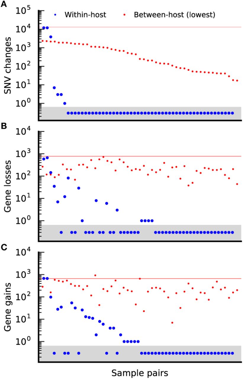
(a) Number of detected nucleotide differences in core and accessory genes between pairs of CP samples from the same host at two consecutive timepoints (blue circles), sorted in descending order. Pairs with zero detected changes are assigned an arbitrary value < 1 (grey region) so that they can be visualized on the logarithmic scale. For comparison, the 50 lowest values from the between-host distribution (red points) and the median between-host value (solid red line) are included as a control. (b,c) the number of gene losses (b) and gains (c) for the sample pairs in (a), listed in the same order. The dashed line again denotes the median between-host value in both cases, while the red points show the corresponding gene losses (b) and gains (c) for the between-host comparisons in (a), plotted in the same order.
The total number of SNV modifications in Fig. 5 is small, making it difficult to tell whether these changes reflect selection on de novo mutations or introgression from other species or lineages (62). We can gain more insight into this question by investigating the gene content differences between timepoints (Fig. 5B,C). The gene losses in Fig. 5B could have been generated by mutations (e.g. large deletion events) or by horizontal exchange (e.g. recombination with a homologous fragment where the genes have already been deleted). By contrast, the gene gains in Fig. 5C must be pre-existing variants, likely acquired through recombination with another lineage. However, we cannot exclude more elaborate clonal scenarios, e.g. a gene deletion that nearly sweeps to fixation in one timepoint, but is later outcompeted by the ancestor in a second timepoint.
Compared to the SNV distribution in Fig. 5A, more of the individuals show evidence for at least one gene difference in Figs. 5B,C, and the average number of differences per individual is slightly higher. The genes that are gained and lost tend to be drawn from the accessory portion of the B. vulgatus genome (Fig. S11A), consistent with the expectation that these genes are more likely to be gained or lost over time. Within a single host, gene changes tend to be spatially clustered along the reference genome in which they are found, suggesting that multiple genes may be altered in a single gene-change event (Fig. S11B). Similar patterns are observed in sequenced isolates (63) and metagenomes from different hosts (59). Thus, the number of introgression events may be significantly lower than the number of gene changes in Figs. 5B,C.

Left: Distribution of gene prevalence (fraction of hosts with copy number ≥ 0.3) for all genes (black), genes that differ between hosts (red), and genes that differ within hosts over time (blue). All calculations are restricted to the samples used in Fig. 5. Middle: Distribution of fold change in copy number for genes immediately upstream and downstream of genes that differ within hosts over time (blue), a randomly selected gene (black), or genes that differ between hosts (red). Definitions of upstream and downstream are based on genome coordinates of the isolates used to construct the pangenome (47). in the isolate used to construct the in which the target gene is found. Right: Distribution of the largest fold change of a given gene in another individual for genes that differ within hosts over time (blue), randomly selected genes (black), or genes that differ between hosts (red).
The patterns observed in Fig. 5 are not unique to B. vulgatus, but are also recapitulated in many of the other prevalent species as well (Fig. S12). We can therefore gain more information about the tempo and mode of adaptation by pooling within-host changes across different species and hosts (Fig. 6). In this larger sample, we see that outright replacement events are relatively rare over the ~ 6 month sampling window (≈ 5% of host-species pairs), though they would dominate the average number of within-host SNV differences if we did not exclude them (Fig. 6A). Below this replacement threshold, ≈ 20% of host-species pairs acquire a modest number of SNV modifications between the two timepoints. These SNV differences are evenly split between “mutations” away from the consensus allele across the panel, or “reversions” back toward it (Fig. 6D). The proportion of reversions is significantly higher than expected for a randomly selected site, and is closer to the distribution of between-host differences. In addition, there are fewer nonsynonymous mutations within hosts than one would expect for neutral or positively-selected sites (dN/dS ≈ 0.4, Fig. 6C). Instead, the fraction of nonsynonymous mutations is shifted towards the between-host distribution in Fig. 3D, even though we expect few deleterious mutations to be efficiently purged on ~ 6 month timescales. The excess of SNV reversions and low dN/dS, combined with the high fraction of gene gains in Fig. 6E, suggest that many of these SNV differences are likely acquired via introgression from another species or strains. In this case, natural selection could have had more time to purge deleterious variants on the introgressed fragment, resulting in the lower fraction of nonsynonymous mutations observed in Fig. 3D. Although lower than expected for de novo mutations, the fraction of nonsynonymous mutations is still slightly higher than in a typical between-host comparison. These extra nonsynonymous mutations could be consistent with a small fraction of de novo driver or passenger mutations, as well as a preference toward introgression from more closely related strains.

Summary of within-host SNV changes (top) and gene changes (bottom) across all species with at least 5 pairs of longitudinal CP samples. Each row in each bar represents a different longitudinal pair, and rows are colored according to the total number SNV changes (top) and gene changes (bottom), with grey indicating no detected changes. A star is included if the total number of non-replacement changes is ≥ 10 times the total estimated error rate across samples (see SI Sections 3.4 and 3.5), where replacements are defined as in Fig. 6.

(a) Within-host nucleotide differences over ~ 6 months. The blue line shows the distribution of the number of SNV differences between consecutive timepoints for different species and CP hosts; species are only included if they have at least 5 consecutive CP timepoint pairs, and pairs with zero detected changes are assigned an arbitrary value < 1 so that they can be visualized on the logarithmic scale. For comparison, the distribution of the closest between-host differences for each initial timepoint is shown in red. The grey region indicates an ad-hoc threshhold used to define replacement events in panels (b-e), chosen to be conservative in calling non-replacements. (b) Within-host gene content differences (gains+losses) in non-replacement timepoints. The blue line shows the distribution of the number of gene content differences between consecutive timepoints for different species and CP hosts; replacement timepoints (those with SNV differences in the grey region of panel A) are excluded. The between-host expectation is the same as in (a). (c) The total number of nucleotide differences at non-degenerate nonsynonymous sites (non) and fourfold degenerate synonymous sites (syn) for the non-replacement species-host combinations in (a). The observed values are indicated in blue. For comparison, we have also included the expected distribution of de novo mutations (randomly selected sites, grey) and between-host differences (red), conditioned on the same total number of events. (d) The total number of nucleotide differences that transition away from the panel-wide consensus allele (mut) and back toward the consensus allele (rev) for the non-replacement species-host combinations in (a). Between-host and de novo expectations are the same as in (c). (e) The total number of gene loss and gain events among the gene content differences in (b). The between-host expectation is the same as in (d), while the de novo expectation is 100% losses.
In the pooled data, gene changes are again more prevalent than SNVs, with ~ 30% of host-species pairs showing some gene-content differences between timepoints (Fig. 6B). Many of these genes are annotated as transposons, integrases, transferases, and mobilization proteins (Table S3), consistent with the hypothesis that they originated through recombination. Similar conjugative elements have been associated with transfers between different Bacteroidales species that colonize the same host (63). We also observe a handful of gene changes in other functional categories (e.g. transcriptional regulators, transmembrane proteins, and ABC transporters). Similar categories are found for genes that harbor SNV differences over time (Table S4). However, the vast majority of genes in both cases are unannotated. Further investigation of the functional parallelism of within-host changes remains an interesting avenue for future work.
DISCUSSION
Evolutionary processes can play an important role in many microbial communities. Yet despite increasing amounts of sequence data, our understanding of these processes is often limited by our ability to resolve evolutionary changes in populations from complex communities. In this work, we have attempted to quantify the evolutionary forces that operate within bacteria in the human gut microbiome, based on a more detailed characterization of the lineage structure in metagenomic samples from individual hosts.
Building on previous work by Truong et al. (40) and others, we found that the lineage structure in many prevalent species is consistent with colonization by a few distinct strains from the larger population, with the identities and frequencies of these strains varying from person-to-person (Fig. 1). The distribution of strain frequencies in this “oligo-colonization model” is quite interesting. In the absence of fine tuning, it is not clear what mechanisms would allow for a second or third strain to reach intermediate frequency, while preventing a large number of other lineages from entering at the same time. A better understanding of the colonization process, and how it might vary among the species in Fig. 1F, is an important avenue for future work.
Given the wide variation among hosts, we chose to focus on a subset of samples with particularly simple strain mixtures, in which we could resolve evolutionary changes in the dominant lineage with a high degree of confidence. Our approach can be viewed as a refinement of the “consensus approximation” employed in earlier studies (4, 36, 39, 40), but with more quantitative estimates of the errors associated with detecting genetic differences between lineages in different samples.
By analyzing the genetic differences between lineages in separate hosts, we found that the long-term evolutionary dynamics of many gut bacteria are consistent with quasi-sexual evolution and purifying selection, with relatively weak geographic structure. The relatively high rates of fine-scale recombination (r ≳ 0.1µ) are qualitatively similar to several bacterial species (14, 64, 65, 66, 67, 68), though the decay of linkage disequilibrium diverges from the standard neutral prediction. By leveraging the two-level population structure in the microbiome, we also uncovered evidence for additional genealogical processes operating at very short timescales, with altered signatures of selection (Fig. 3) and potentially recombination as well (Fig. S10). It is difficult to produce such a broad range of core-genome-wide divergence in existing population genetic models, given the homogenizing effects of recombination, though recent hybrid models of vertical and horizontal inheritance may provide a potential explanation (68, 69). Our findings suggest that this may be an interesting signature to explore in future theoretical work, in addition to further empirical characterization in larger cohorts and over shorter genomic distances. In either case, the present findings suggest that the short-term dynamics of across-host evolution may not be easily extrapolated by comparing sequences of typical isolates.
With quantitative estimates of the false positive rate, our approach is also capable of resolving a smaller number of SNV and gene changes that could accumulate within hosts over time. This allowed us to build on previous findings that personal microbiomes are largely stable over time (33, 40, 46, 47, 59, 60), to start to quantify the tempo and mode of evolution within individual hosts. Consistent with this earlier work, we only observe a few replacement events in which the dominant lineage is succeeded by a strain as distantly related as those in other hosts. Given the existing data, it is difficult to tell whether these replacements are due to the invasion of a new lineage, or a sudden rise in frequency of an existing lineage. Deeper sequencing coverage could potentially show whether the new lineage was already present at the initial timepoint (as in Fig. S13A), though this could also be consistent with a slow sweep by an invading lineage. These scenarios could potentially be distinguished with additional time series data, since a preexisting lineage could re-emerge in later timepoints (23). One such reversal occurred in one of the B. vulgatus individuals sampled at three timepoints (Fig. S13A).

SNV frequency trajectories (a-c) and gene copy number trajectories (d-f) as a function of visit number for three example host/species combinations (left, center, and right). Each line represents a different SNV or gene variant, and the lines are colored for visualization. In (a-c), allele frequencies are polarized according to the first visit number, and SNVs are only included if they have frequency ≤ 20% at the first timepoint, and ≥ 80% at one of the later timepoints (dashed lines). SNVs are excluded if they fail to meet the coverage requirements at any of the three timepoints. In (d-f), genes are only included if the initial copy number lies in either the present or absent regions (illustrated by dashed lines), and if at least one later timepoint is in the opposite state. Genes are excluded if they exceed the maximum copynumber (c ≤ 2) at any of the three timepoints.
Although rare replacement events account for the bulk of all within-host SNV changes, we more commonly observed lineages that differed by only a handful of SNV and gene changes, suggestive of an evolutionary modification (Fig. 6). This shows that it is important to consider the full distribution of temporal changes, since species-averaged (40, 46) or metagenome-averaged (33) estimates are dominated by the rare replacement events. Although it is possible that the putative modifications could result from replacement by an extremely closely related strain, we believe that this scenario is less likely, since it requires circulating strains that are more closely related than even the lower tail of the between-host distribution (Fig. 5), and with dN/dS values somewhat lower than expected from Fig. 3D. However, unambiguous proof of a modification could potentially be observed in a longer timecourse, since subsequent modifications should eventually accumulate in the background of earlier substitutions. Based on our limited data, we can already observe a few examples of this behavior in individuals sampled at three timepoints (Fig. S13B,C).
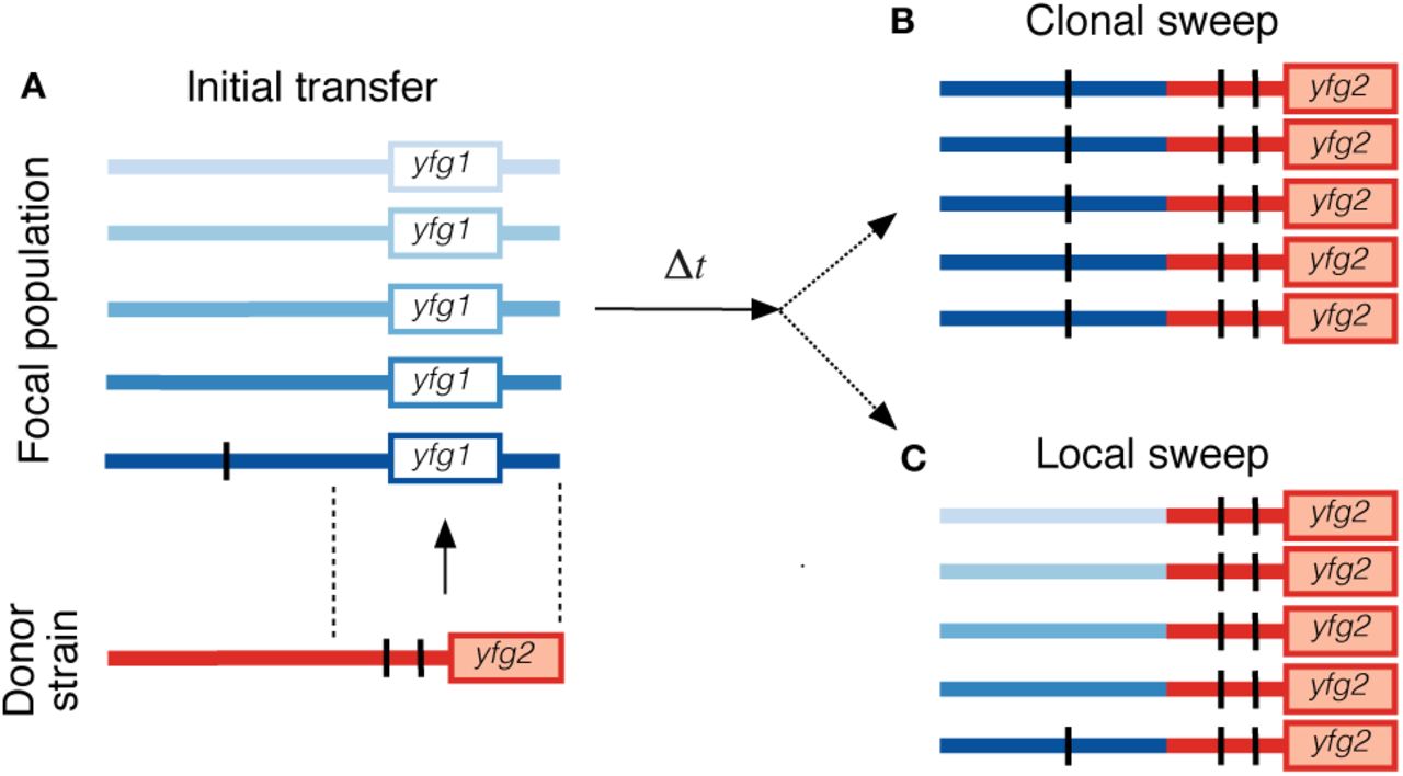
Many of the mutations we observed are gene gain events, which, combined with the signatures of the sweeping SNVs (Fig. 6), suggests that SNV and gene modifications are often acquired via introgression from an existing strain (illustrated in Fig. 7A). This stands in contrast to the de novo mutations observed in microbial evolution experiments (11) and some within-host pathogens (19, 20). Yet in hindsight, it is easy to see why adaptive introgression could be a more efficient route to adaptation in a complex ecosystem like the gut microbiome, given the large strain diversity (44), the high rates of DNA exchange (70, 71), and the potentially larger selective advantage of importing an existing functional unit (9). Consistent with this hypothesis, adaptive introgression events have also been observed on slightly longer timescales in bacterial biofilms from an acid mine drainage system (12), and they are an important force in the evolution of virulence and antibiotic resistance in clinical settings (72).

(a) A hypothetical introgression event, in which a new gene (yfg2) and two SNVs (black lines) are transferred from a donor strain (red) into a single individual in the focal population (blue, each individual is assigned a unique shade). In addition to the gene gain and SNV substitutions, this introgression event also results in the loss of the existing gene yfg1 in the introgressed individual. (b) An example of a clonal sweep, in which the initial recombinant in (a) sweeps to fixation in the focal population, resulting in a within-host gene gain (yfg2), a gene loss (yfg1), and 3 SNV changes (2 on the introgressed fragement, 1 de novo variant). (c) An example of a clonal sweep, in which the introgressed fragment is able to recombine onto other genetic backgrounds before it reaches fixation. Note that the private variant no longer hitchhikes to fixation.
While the data suggest that within-host sweeps are often initiated by a recombination event, it is less clear whether recombination is relevant during the sweep itself. Given the short timescales involved (~ 6 months), and our estimates of the recombination rate (r ≳ 0.1µ; Fig. S9), we would expect many of the observed sweeps to proceed in an essentially clonal fashion (Fig. 7B), since recombination would have little time to break up a megabase-sized genome. If this were the case, it would provide many opportunities for substantially deleterious mutations (with fitness costs of order Sd ~ 1% per day) to hitchhike to high frequencies within hosts (25), thereby limiting the ability of bacteria to optimize to their local environment. The typical fitness costs inferred from Fig. 3D lie far below this threshold, and would therefore be difficult to purge within individual hosts. In this scenario, the low values of dN/dS observed between hosts (as well as the putative introgression events) would crucially rely on the competition process across hosts (73).
Although the baseline recombination rates suggest clonal sweeps, there are other vectors of exchange (e.g. transposons, prophage, etc.) with much higher rates of recombination. Such mechanisms could allow within-host sweeps to behave in a quasi-sexual fashion, preserving genetic diversity elsewhere in the genome (Fig. 7C). These “local” sweeps are occasionally observed in other bacterial systems (13, 15). If local sweeps were also a common mode of adaptation in the gut microbiome, they would allow bacteria to purge deleterious mutations more efficiently than in the clonal scenario above.
In principle, we can distinguish between clonal and local sweeps by searching for SNV substitutions in non-CP samples, and checking whether diversity is maintained at other loci after the sweep. Although we must employ more stringent criteria to detect sweeps in these non-CP samples, we can find a few individual examples of putatively clonal and local behavior (Fig. S14, SI Section 7). However, in the latter case, it is difficult to distinguish a true local sweep from a clonal event in a gene that is present in only one of the lineages in the host. In this case, we would require longer-range linkage information (41) to determine whether the sweeping alleles are present in multiple strains.

(a-c) Final vs initial allele frequencies for all SNVs in the B. vulgatus genome in three pairs of longitudinal samples whose initial timepoint was classified as non-CP. Allele frequencies are polarized such that the change in allele frequency is positive. In each panel, SNVs are colored if they are in a gene with at least two detected SNV changes that are more than 100bp apart, with each gene assigned its own color. All other SNVs are colored grey. SNVs are only plotted if they had sufficient coverage at both timepoints, and if at least one timepoint had allele frequency ≥ 0.05. Panel (a) illustrates a putatively clonal sweep, while panels (b) and (c) suggest local sweeps. (d) The distribution of relative coverage at all core-genome sites at the initial timepoint in panel (b). The median coverage for the colored sites in (b) is indicated with the corresponding line and symbol. (e) An analgous version of (d) for the individual in panel (c). Note that in both (d) and (e), the sweeping genes are outliers in the coverage distribution.
While we have identified many interesting signatures of within-host adaptation, there are several important limitations to our analysis. First, our reference-based approach only allows us to track SNVs and gene copy numbers in the genomes of previously sequenced isolates of a given species. Within this subset, we have also imposed a number of stringent bioinformatic filters, further limiting the sequence space that we consider. Thus, it is likely that we are missing many of the true targets of selection, which might be expected to be concentrated in the host-specific portion of the microbiome, multi-copy gene families, or in genes that are shared across multiple prevalent species. A second important limitation of our approach is that it can only identify complete or nearly complete sweeps within individual hosts. While we observed many within-host changes that matched this criterion, we may be missing many other examples of within-host adaptation where variants do not completely fix. Given the large population sizes involved, such sweeps can naturally arise from phenotypically identical mutations at multiple genetic loci (74, 75), or through additional ecological partitioning between the lineages of a given species (23). Both mechanisms have been observed in experimental populations of E. coli adapting to a model mouse microbiome (6).
Our present observations do not uniquely determine the population genetic models that describe evolution in the gut microbiome. However, we have shown that they place a number of strong constraints on this process, sufficient to rule out many of the simplest explanations of the data. We hope that these constraints provide a useful starting point for additional theoretical and empirical studies to advance our understanding of evolution in the microbiome.
SUPPLEMENTAL TABLES
TABLE S1 Metagenomic samples used in study. We analyzed 1576 samples from the Human Microbiome Project (HMP), and 185 samples from Qin et al. (45). Listed are the subject ids, sample ids, run accessions, country of the study, continent of the study, visit number, and study (HMP or Qin et al, 2012).
TABLE S2 Top-level clade definitions. This table contains the manually-defined top-level clades described in SI Section 4.1. Rows list the various combinations of species and hosts plotted in Fig. 3, along with its corresponding numeric clade label.
TABLE S3 Gene change annotations. All genes that changed across the species analyzed in Fig. 6B were annotated with the PATRIC (76) database. Several genes were grouped into a single category based on keyword matches as described in SI Section 8. Listed are the total number of gene changes, the expected number of changes assuming a null comprised of all changes between hosts, a null comprised of all genes present in hosts at all time points, and a null comprised of genes present in the pangenome. Expectations are also listed for gene gains and loss using the same three nulls. Lastly, the names of genes that are grouped together in a single keyword category are listed.
TABLE S4 SNV change annotations. An analogous version of Table S3 for genes that harbored a within-host SNV change. Listed are the total number of genes with at least one SNV change between consecutive timepoint pairs, and the expected number of hits under a null comprised of all changes between hosts and a null comprised of all genes present in hosts at all time points. Lastly, the names of genes that are grouped together in a single keyword category are listed.
SUPPLEMENTAL INFORMATION
1. VARIANT CALLING
We analyzed whole-genome sequence data from a panel of 499 stool samples from 365 healthy human subjects (Table S1). Of these, 185 samples from China (all unique subjects) were previously sequenced by Qin et al. (45), and 314 samples from North America were from 180 subjects from the Human Microbiome Project (44) (87 individuals sampled once; 52 sampled 2 times roughly 6 months apart; 41 individuals sampled 3 times over the span of ~ 1 year). Previous work has shown that there is little genomic variability between technical and sample replicates in HMP data (46, 47), so we merged fastq files for technical and sample replicates from the same time point to increase coverage to resolve within-host allele frequencies.
We analyzed these samples using the MIDAS software package [v1.2.2 (47)], with custom filters and postprocessing scripts. MIDAS first quantifies the relative abundances of species in different metagenomic samples by mapping sequencing reads to a database of universal, single-copy “marker” gene sequences using HS-BLASTN (77). Based on this step, species with average marker gene coverage ≥ 3 are defined as “present” in a given sample. These species are then concatenated to create a sample- specific reference genome and corresponding reference pangenome for the SNV and gene content estimation steps using the default MIDAS database (version 1.2, downloaded on November 21, 2016). To minimize potential mapping artifacts in detecting changes in longitudinally sampled individuals, we counted a species as present in all timepoints for a given individual if it was deemed present in any single timepoint, and this larger set of species was used to construct a consistent set of reference genomes and pangenomes across the different timepoints.
1.1. Quantifying gene content
To quantify gene content in each sample, sequencing reads were aligned to the sample-specific pangenome using Bowtie2 (78) with default MIDAS settings: local alignment, MAPID ≥94.0%, READQ ≥20, and ALN_COV ≥0.75. We note that with these settings, reads with multiple best-hit alignments will be distributed among these targets according to their proportional representation on the pangenome reference sequence.
For each species, average coverage was reported for each gene after clustering at 95% sequence identity, as well as for a panel of universal, single-copy marker genes (47). Gene content was only evaluated in species with marker coverage ≥ 20 in a given sample. The ratio between gene and marker coverage was used to estimate the copy number of each gene in the sample. We used this information to define a “core genome” for each species, defined as the set of all genes with copy number ≥ 0.3 in ≥ 90% of hosts in our panel. All other genes were defined to be “accessory” genes.
Given the limitations of our short-read approach, we cannot definitely prove that a read came from a particular species, particularly in the case of highly conserved or highly promiscuous genes. We therefore restricted our downstream analyses to genes with copynumbers in the range 0 ≤ c ≤ 0.05 (“absent”) and 0.5 ≤ c ≤ 2 (“present”), in order to reduce potential cases where fluctuations in species abundance would lead to erroneous gene content changes. In principle, sequence data with longer-range linkage information (41) could be used to confirm that any gene content differences are linked with the appropriate core-genome backbone.
1.2. Identifying SNVs
To identify putative SNVs, sequencing reads were aligned to sample-specific reference genomes using Bowtie2, with default MIDAS mapping thresholds: global alignment, MAPID ≥94.0%, READQ ≥20, ALN_COV ≥0.75, and MAPQ ≥20. After alignment, species were only retained if at least 40% of the reference genome had coverage ≥ 1. MIDAS reports reference and SNV allele counts using samtools mpileup (79). We defined the within-sample allele frequency to be the fraction of reference alleles at a given site. (When present, multiple alternative alleles are therefore merged into a single allele.)
For each species, we then calculated the distribution of coverage at all sites in the core genome in each sample. We used this information to define a characteristic coverage value  for each sample, defined as the median of all core genome sites with nonzero coverage. To ensure adequate coverage for accurately estimating allele frequencies, samples with
  < 20 were excluded from further analyses. To further reduce mapping artifacts, sites in a given sample were masked (assigned zero coverage) if their coverage was
  . For similar reasons, we only considered SNVs in coding sequences of annotated genes, and we masked sites with nonzero coverage in fewer than 4 samples across our panel.
When comparing groups of samples, we defined a site to be a potential SNV candidate if it had within-host frequency > 5% in at least one sample. To avoid including sites due to rounding biases, we stipulated that the frequency must exceed 5% by at least 1/D. All other sites were assumed to be monomorphic in that comparison. When analyzing a single sample (e.g. in Figs. 1A-D and SI Section 3.2), all sites were included regardless of allele frequency.
2. WITHIN-HOST EVOLUTION IN A SINGLE-COLONIZATION MODEL
In this section, we further explain the assumptions made in computing the expected within-host polymorphism rate for a given species under a simple, single-colonization model. As described in the text, we will make conservatively high estimates for the per site mutation rate (µ ~ 10−9 per generation), generation times (λ ~ 10 generations per day), and time since colonization (∆t ~ 100 years). We define the within-host polymorphism rate P as the fraction of fourfold-degenerate synonymous site mutations with allele frequencies in the range 0.2 ≤ f ≤ 0.8. In the single-colonization model, the mutations that contribute to P must have reached intermediate frequencies after starting as a de novo mutation at some time after colonization.
We assume that the synonymous mutations are effectively neutral over the timespans considered (sλ∆t ≪ 1). Under this assumption, one of these mutations can only contribute to P if it hitchhiked along with a lineage that rose to a frequency in the range 0.2 ≤ f ≤ 0.8. This can happen either due to neutral drift (i.e., the lineage randomly fluctuated to intermediate frequencies) or selection (i.e., the lineage reached intermediate frequencies because it contains a beneficial mutation). However, if synonymous mutations are neutral, their presence or absence in a lineage is independent of the processes that drive it to intermediate frequency (80). The probability that a particular neutral mutation arose along the line of descent is simply the product of the per-site mutation rate µ and the total number of generations since the lineage diverged from the common ancestor between it and the rest of the population. By assumption, the latter is bounded by the total number of generations since colonization (λ∆t). This yields the conservative estimate for the within-host polymorphism rate,
 quoted in the main text.
3. PHASING METAGENOMIC SAMPLES
In this section, we describe the methods used to estimate one of the dominant haplotypes in a subset of the metagenomic samples (the confidently phaseable (CP) samples), and to quantify genetic differences between these lineages. The method is similar in spirit to recent work by Truong et al. (40), but with a greater emphasis on estimating the associated false positive rates.
3.1. Theoretical motivation
To gain intuition for how within-host lineage structure is reflected in the distribution of allele frequencies, it is useful to start by considering the simplest version of the phasing problem, in which the metagenomic reads for a given species in a particular sample are derived one of two clonal lineages mixed in a proportion fmix ≥ 50% (representing the proportion of cells from the more abundant lineage). Within-sample polymorphisms will arise from fixed differences between the two lineages and will segregate at frequency fmix or 1 − fmix, depending on which lineage the mutation arose in and the choice of reference allele. Since this choice is arbitrary, we work with the major allele frequency in each sample. In this case, the distribution of major allele frequencies, p(f), will then have the simple form
 where d is the average nucleotide divergence between the two lineages and δ(z) is the Dirac delta function. Note that this theoretical distribution is only obtained in the limit of infinite coverage; in practice, the observed distribution of major allele frequencies will be blurred due to sampling noise (see SI Section 3.2 below). Nevertheless, in the the limit of high coverage, Eq. (S3.1) suggests that we can infer fmix and d by looking for a peak in the distribution of major allele frequencies (e.g., Fig. 1E). Again, in the idealized case, the two haplotype sequences are easy to recognize: major alleles are assigned to the dominant lineage, while the minor alleles belong to the subdominant type.
This basic idea also extends to mixtures of more than two lineages, but the potential genealogical relationships between them make the problem much more complicated. For example, in a mixture of three strains with frequencies f1, f2, and f3, the distribution of major allele frequencies will now have three characteristic peaks (corresponding to min{fi, 1 − fi} for each i = 1, 2, 3). This time, however, alleles that segregate at the same frequency do not necessarily belong to the same lineage, since they could also be ancestral to two of the three strains. There are three possible genealogies relating the three strains, which can vary from site-to-site in the presence of recombination. Haplotype estimation then becomes a complicated inference problem, which only grows more difficult as additional lineages are added. Consideration of the combined allele frequency distribution may be helpful for deriving error models for algorithms that attempt to deconvolute strains from metagenomes.
Rather than trying to infer the exact mixture proportions and the haplotypes of each lineage, we developed a set of heuristic rules to identify the haplotype of just one of the dominant lineages while controlling the probability of misassigning variants to this haplotype. Suppose that there are within-sample polymorphisms at two sites, with major allele frequencies f1 and f2. We denote the four (unobserved) two-locus haplotype frequencies by fMM, fMm, fmM, and fmm, where M and m denote the major and minor allele at each site. If f1 = f2 = 0.5, then there are no constraints on the possible haplotype frequencies, other than the marginal constraints fMM + fMm = f1 and fMM + fmM = f2. However, in the opposite extreme where f1 = f2 = 1, then normalization constraints require that fMM = 1 (i.e., the major alleles are on the same haplotype). In between these two extremes there is a more general rule that, whenever the allele frequencies satisfy fi ≥ f, with log(f/1 − f) = c ≳ 1, the minimum possible frequency of the MM haplotype is

Equation S3.2 represents a worst case scenario in which the haplotypes are specifically assigned to prevent major alleles from segregating together. In practice, a more realistic lower bound for the fM M is attained when the alleles are in linkage equibrium:
 which happens to have the same asymptotic behavior in this two-locus example. In either case, these bounds show that an appreciable fraction of cells in the host must possess both major alleles.
This argument can also be extended to larger collections of sites. In the pessimistic case of linkage equilibrium between all polymorphic sites, the number of major alleles per individual is binomially distributed with success probability f. In the limit of a large number of sites, this means that the vast majority of the cells will have the major allele at a fraction f of the possible sites. However, while the haplotype consisting of all major alleles is the most likely haplotype under linkage equilibrium, its expected frequency can grow quite small, to the point where the haplotype may not even be present in a finite sample. Fortunately, our analysis will primarily focus on one- and two-locus statistics where the stronger bounds in Eq. (S3.2) can be applied.
3.2. False positive rate for SNP phasing
The arguments above suggest that, for many downstream purposes, we can effectively estimate a portion of one of the haplotypes in a metegenomic sample by taking the major alleles present above some threshold freuqency, f * 50%, and treating sites with intermediate frequencies as missing data. This is a simple generalization of the consensus method (i.e. taking the haplotype formed by all major alleles) that has been used in previous metagenomic studies (4, 40), and it is similar to methods used to genotype clonal isolates from whole-genome resequencing data (81).
The major difficulty with this approach is that we do not observe the true frequency f directly, but rather a sample frequency  that is estimated from a finite number of sequencing reads. Polarization errors (i.e. errors in determining the major allele) can therefore accumulate when the allele supported by the most reads differs from true major allele in the sample. When sequencing clonal isolates, such false positives are primarily caused by sequencing errors. These occur at a low rate per read (perr ~ 1% per bp), and become increasingly unlikely at moderate sequencing depths. However, in a metagenomic sample, polarization errors will also arise due to finite sampling noise, when an allele at some intermediate frequency (e.g. 25%) happens to be sampled in a majority of the sequencing reads. As we will show below, for moderate sequencing depths, this will often be the dominant source of error.
To model this process, let Aℓ, Dℓ denote the number of alternate alleles and total sequencing depth at a given site ℓ in the genome, and let  denote the corresponding sample frequency. We assume that the number of alternate reads follows a binomial distribution,
 for some true frequency fℓ, so that the probability of observing
  is simply

A polarization error will occur when we observe  even though fℓ < 50%. Equation (S3.5) shows the probability of such an error will strongly depend on fℓ. For a sequencing depth of D = 10 and a frequency threshold of f ∗ = 80%, the error probability ranges from essentially negligible (∼ 10−14) when f is on the order of the sequencing error rate (∼ 1%), to ∼ 1 per bacterial genome when f ≈ 10%, to an error rate of 5% when f ≈ 50%.
The average false positive rate across the genome will therefore depend on an average over the possible values of f and D:
 where p0(D, f) is the prior distribution of D and f at a randomly chosen site (Fig. S1A). In the absence of any additional information, this joint distribution with the product of empirical distributions,
 which we estimate for a given sample by binning the observed values of D and the allele frequencies across the L sites under consideration (blue distribution in Fig. S1A). The expected number of polarization errors in a given sample across all L sites is given by

This calculation holds for any large collection of sites where the empirical distribution,  , provides a reasonable approximation to the prior distribution, p0(f). For example, in the following section, we consider the set of all synonymous sites in the core genome.
3.3. Confidently phaseable samples
The basic idea behind our approach is that we wish to restrict our attention to samples where Nerr is small compared to the total number of sites under consideration. This number will vary depending on the particular analysis that we wish to carry out. But for population-genetic purposes, it will always be related to the number of sites that actually vary between samples. As a simple proxy for this number, we therefore consider a measure of the average genetic distance between the dominant haplotype in a given sample and the lineages in the remainder of our panel.
Specifically, we focus on fourfold-degenerate synonymous sites in the core genome. For each sample, let N< denote the number of such sites with major allele frequencies less than f∗, and conversely, let N> denote the number of sites with  . For the sites in the latter group, let
  denote the corresponding allele frequency across the entire panel. Then the quantity
 approximates the expected number of differences at these sites for an “average” individual drawn from the panel. A normalized version (Nd/L) is illustrated for the B. vulgatus samples in Fig. S2. We declare the sample to be a confidently phaseable (CP) sample if it passes the coverage thresholds in SI Section 1 and N</Nd < 0.1.
To see why this is a reasonable definition, we return to our error formula in Eq. (S3.8) and plug in conservative estimates for p0(D, f). For example, we expect that the number of truly polymorphic sites in the sample will also be of order ∼ Nd, with the remaining sites having frequencies near the sequencing error threshold, f ∼ 1%. We then divide the remaining polymorphic sites into the fraction N</Nd ≲ 0.1 with major allele frequencies below f∗, and the remaining fraction (∼ 100%) with major allele frequencies above f∗. If we make the conservative approximation that all of the sites in the latter group have minor allele frequencies f ≈ 1 − f∗, and all of the sites in the former group have f ≈ 50%, then we obtain an approximate prior distribution for f :

If we make a similarly conservative approximation for the coverage distribution,
 where δ is the Dirac function, then for a threshold of f∗ = 80%, the realized false positive rate is

Thus, with these thresholds, we expect that only a small fraction of informative sites (as defined by the average distance between samples) will be susceptible to polarization errors.
3.4. False positive rate for SNV differences
Although the CP sample classification is a good rule of thumb for determining when polarization errors are more or less likely to happen, there are scenarios where we wish to measure genetic distances between samples (e.g. longitudinal samples from the same individual) that are much more closely related than an average pair of individuals in our panel. In these cases, the realized false positive rate can be much higher than the estimate in Eq. (S3.12). To obtain more accurate estimates of the error in these cases, we extend our calculation above to the specific problem of detecting the number of nucleotide differences between two samples.
Generalizing from the phasing problem above, we would conclude that the haplotypes in two samples share the same allele at a given site if that allele is present above frequency f∗ in both samples. To observe a difference between the two samples, the allele would have to be present above frequency f∗ in one sample and below 1 − f∗ in another. If the allele lies between 1 − f∗ and f∗ in one of the samples, the site is treated as censored data. Under this definition, a nucleotide difference requires a change in allele frequency of at least

If we rewrite everything in terms of ∆ f, a nucleotide difference requires the allele frequency to lie below (1 − ∆f)/2 in one sample and above (1 + ∆f)/2 in another (pink shaded regions in Fig. S1B). We will adopt the latter notation here, as it allows us to easily consider more stringent thresholds for which ∆f > 2f∗ − 1.
Under the null hypothesis, we assume that the true allele frequency f is the same in the two samples. If we let D1 and D2 denote the coverage of the site in the two samples, then a simple generalization of Eq. (S3.6) shows that the false positive rate for a randomly chosen site is given by
 where
where  is defined in Eq. (S3.5) and p0(D1, D2, f) is the prior distribution for D1, D2, and f at a random site. As in Eq. (S3.7) above, we estimate this prior distribution as a product of empirical distributions,
 which we estimate by binning the observed values of D1, D2, and
  across the genomes of the two samples (the blue distribution in S1B). The expected number of false positive substitutions is then given by
 where L is the total number of sites compared between the two samples. This will vary depending on the application (e.g. synonymous sites, sites in core genes, all coding sites, etc. are used at various times in the main text).
The error estimate in Eq. (S3.16) is an implicit function of the threshold ∆ f. Given the typical sequencing coverages and allele frequency distributions of the CP samples in our analyses, we usually obtain sufficiently low error estimates (i.e., Nerr ≪ 1) if we take ∆f = 1 − 2 f ∗ = 0.6, so that an allele transitions from less than 20% to greater than 80% frequency between the two samples, or vice versa. However, for the few outlier sample pairs where Nerr > 0.5, we attempted to increase ∆ f until Nerr(∆f ≤ 0.5. If this was not possible, we discarded that pair of samples from further analysis.
3.5. False positive rate for gene content differences
The false positive rate for gene content differences can be estimated with a similar procedure. In this case, the canonical generative model is one in which a gene g with average copy number per cell cg,i in sample i recruits Ng,i reads, which we assume follows a Poisson distribution:
 where Lg is the length of gene g and Fi is a sample- and species-specific constant that reflects the total number of reads aligned to that species (e.g., by the MIDAS pipeline). The coverage of gene g is then defined as
 where Lr,i is the average length of reads that align to that gene (typically ≲ 100bp), which can vary in a sample-specific manner. The quantity ℓg,i = Lg/Lr,i then serves as a conversion factor between the raw number of reads and the coverage. Finally, we assume (as in the MIDAS pipeline) that there is a known panel of marker genes (g = m) with fixed copy number per cell of cm ≈ 1 and a large target size, such that
  . This allows us to eliminate Fi and rewrite Eq. (S3.17) in terms of the marker coverage Dm,i and the coverage-to-read conversion factor ℓg,i:

The variables Ng,i, Dg,i, and Dm,i are all reported by MIDAS, which allowed us to estimate cg,i and ℓg,i for each gene in each sample:

Based on the above error rate calculations, the gene copy number change events we are interested in are those in which a gene transitions from a “typical” copy number value (0.5 ≤ c ≤ 2, see Fig. S6) in one sample to a value close to zero (c < 0.05) in another. This does not cover all possible copy number change events, but focuses on the subset that are likely to be (i) statistically significant and (ii) less susceptible to other bioinformatic errors (e.g. read stealing or donating from other species).
Given this definition, the probability of an apparent copy number change happening by chance will again depend on the “true” copy number of the gene, c, as well as its effective coverage, ℓD. Similar to Eq. (S3.14), the expected false positive rate for a randomly chosen gene is given by
 where FP(k; λ) is the Poisson CDF and p0(ℓ, c) is the null distribution of ℓ and c. Once again, we estimate this joint distribution with the product of empirical distributions,
 which are estimated by binning the observed values of ℓg,i and cg,i across the two samples. To reduce mapping artifacts, we only bin ℓ-values from genes with copy number in the range 0.5 ≤ c ≤ 2, which accounts for the bulk of the copy number distribution in a given sample (S6). The expected number of false positive gene changes is therefore given by
 where npangenome is the total number of genes tested (typically of order ~ 104). For the typical coverages in our dataset, this number is usually very small (≪ 10−2). In the few cases where the coverage is sufficiently low that Nperr > 0.5, we discarded the sample pair from consideration.
4. POPULATION STRUCTURE ACROSS HOSTS
In this section, we describe the methods used to analyze the population structure of a given species based on between-host comparisons.
4.1. Top-level clades
For each species, we constructed core-genome dendrograms by hierarchically clustering the matrix of pairwise divergence rates averaged across the core genome, using the UPGMA method from SciPy (82). Examples for B. vulgatus and B. stercoris are illustrated in Fig. 2. Based on these dendrograms, lineages were assigned to one or more ”top-level” clades using a manual procedure, loosely designed to maximize the difference between inter- and intra-clade divergence at the most deeply diverged branches (Table S2). We adopted this manual procedure to capture clade structure that is inconsistent with a single ‘cut’ through the dendrogram at a given level of divergence.
In Fig. S8A, we plot the fixation index, Fst for these manually defined clades:
 where c indexes the clades and dij is the average nucleotide divergence across core genes in hosts i and j. Several of the prevalent species have top-level clades with high Fst (with B. vulgatus serving as one of the more extreme cases).
4.2. Phylogenetic inconsistency
We quantify potential discrepancies between the core genome dendrograms in Figs. 2A,C and the genealogies of local genomic regions by defining a measure of phylogenetic consistency based on the fraction of homoplasic SNVs (i.e., SNVs that appear to conflict with the core genome dendrogram, see below). Our measure is conceptually similar to recent work by Bobay and Ochamn (83).
For a given core-genome divergence threshold d, we obtain a set of non-overlapping clade groupings C(d) by cutting the UPGMA dendrogram in Fig. 2 at distance d. Then, for each clade c ∈ C(d), we calculate the total number of core-genome sites that are polymorphic within the clade  , as well as the subset that are also polymorphic among the remaining individuals in the population
  . We refer to the latter as phylogenetically inconsistent SNVs, since they are homoplasic at the given level of the genealogy. The net measure of phylogenetic inconsistency in Figs. 2B,D is then defined as the fraction of phylogenetically inconsistent SNVs across all the clades at the given level of divergence:

Note that according to this definition, the same site may be included in the denominator multiple times if it is polymorphic in multiple clades. The same site can also be included for multiple divergence thresholds d.
In general, the overall magnitude of p(d) can be influenced by factors other than the underlying rate of homoplasy. In particular, the probability of observing a phylogenetically inconsistent SNV will strongly depend on its allele frequency, as well as the size distribution of the various clades. To interpret the observed values of p d, we compared them to a null model of free recombination that controls for these statistical biases. For each polymorphic site identified above, we generated a bootstrapped version by permuting the observed alleles across the set of hosts, while requiring that the site remains polymorphic within the clade of interest. This produces a bootstrapped dataset with the same values of  , but with a number of inconsistent sites
  , That reflects the free recombination model. The overall level of phylogenetic inconsistency in this model is then defined as
 and is included as a grey line in Figs. 2B,D.
4.3. Geographic structure
As described in the text, the between-host dendrogram for the Bacteroides vulgatus (Fig. 2A) does not appear to correlate strongly with the geographic location of the hosts. This lies in contrast to some other bacterial species, e.g. Heliobacter pylori (84) which possess more striking patterns of geographic differentiation. To investigate whether this pattern holds in other prevalent gut species, we calculated the fixation index, Fst, between U.S. and Chinese samples using an analgous version of Eq. (S4.1) (with clades replaced by countries). Figure S8 shows the observed Fst values for the set of species in Fig. 3. Apart from E. rectale and E. eligens, these Fst values are relatively low (Fst < 0.1), consistent with previous comparisons between the U.S. and European samples (33). To assess the significance of these Fst values, we compared them to a null model in which the country labels were randomly permuted between the samples. This revealed 5 additional species with lower Fst values (i.e., < 0.1) with P-values less than 0.05 (Fig. S8B).
The Fst statistic can suffer from low power when the two groups are not perfectly partitioned into clades, even if the clades still preferentially harbor hosts from specific countries. To test for such residual geographic structure, we focused on the top-level clades in Table S2. We then asked whether the country of origin was preferentially associated with certain clades. To quantify this tendency, we calculated a likelihood ratio score,
 where
where  and
and  are the observed number of U.S. and Chinese samples in each clade, pc is the expected fraction of U.S. samples in each clade, and
  is the expected fraction of U.S. samples in the entire panel. Only clades with ≥ 2 samples are included in the sum. To focus on the most biologically significant differences, we set

To assess the significance of the observed likelihood ratio scores, we compared them to a null model in which the country labels were randomly permuted between the samples (Fig. S8C). Once again, E. rectale and E. eligens are highly significant, but the remaining species have much weaker signals.
Our analysis is not meant to imply that there is no geographic structure in the species we have considered, but rather that it does not appear to be the main driver of the genome-wide patterns that we observe. There may be additional strongly differentiated clades that were not sampled in our limited panel, or more pronounced geographic structure for genetic differences below our detection threshold. In addition, there may also be strong signals of population structure among individual loci, even if they are averaged out in the genome-wide distances that we consider. More sophisticated methods [e.g. F statistics (85) or programs like STRUCTURE (86)] could be used to investigate this further. These are interesting avenues for future work.
5. POPULATION GENETIC NULL MODEL OF PURIFYING SELECTION FOR PAIRWISE DIVERGENCE ESTIMATES
In this section, we present a minimal model of purifying selection that can account for the varying dN/dS levels in Fig. 3D as a function of dS. The basic idea is that purifying selection is less efficient at purging deleterious mutations that are very young (in particular, younger than the inverse of the associated fitness cost). To the extent that synonymous divergence can be associated with a characteristic timescale, this line of reasoning implies that anomalously low values of dS would be associated with less efficient purifying selection (i.e., higher values of dN/dS), while typical values of dS would be associated with more efficient purifying selection (i.e., lower values of dN/dS). Similar ideas have been employed in previous studies (87, 88).
To make this idea more concrete, suppose that the age of a given mutation is bounded by a time T, so that it occured at some point in the last T generations. This will result in a genetic difference between two randomly sampled lineages with probability
 where N(t) is the population size, f(t; t0) is the frequency of an allele that was created at time t0 and sampled at time t, and the expectation is taken over all possible realizations of f(t, t0). If T is much smaller than the typical coalescence timescale of the population, then the mutation cannot rise to a very high frequency by the time of sampling, and we can neglect the f2 term above to obtain

By definition, the new mutation will arise at frequency 1/N(-t). If the mutation has a deleterious fitness cost s, then its average size is simply
 and we have

If synonymous mutations are assumed to be neutral, we simply have  as expected. If we assume that the nonsynonymous sites have a distribution of deleterious fitness costs ρ(s), then the nonsynonymous divergence rate satisfies

In the simplest case, ρ(s) will contain a mixture of truly neutral mutations and a fraction fd with deleterious fitness cost s, for which

In order to connect this model with the observed data, we must find a way to estimate T. We assume that for anomalously low core-genome-wide divergence rates, the divergence time dS/2µ provides a reasonable estimate of the maximum mutation age T at most polymorphic loci (otherwise, we would expect a more typical value of dS). Based on this assumption, we obtain an empirical relation between dN/dS and dS:
 which is valid for dS much smaller than the population median. For small dS, this ratio will start to deviate from unity when dS ≳ 4µ/sf. At large dS, the ratio approaches 1 − fd, and will start to deviate from this value when dS ≲ 2µfd/s(1 − fd). These landmarks allow us to obtain approximate estimates of fd and s by rough inspection of the data in Fig. 3D.
We note that qualitatively similar behavior is expected in recent models of bacterial evolution proposed by Dixit et al. (68), in which the core genome of closely related strains consists of an asexual ”backbone” (where synonymous mutations occur at rate µ) interrupted by highly diverged segments of length ℓr acquired through recombination. The introgressed segments would enter with low values of dN/dS associated with the average dS value. If the common ancestor of the asexual backbone is younger than the typical deleterious fitness cost, we would again expect a transition from essentially neutral behavior (dN/dS ≈ 1) to the typical between-host value (dN/dS ≈ 0.1) as a function of dS, where the transition is now informative of the horizontal transfer rate. A formal analysis of this model remains an interesting avenue for future work.
6. POPULATION GENETIC NULL MODEL FOR THE DECAY OF LINKAGE DISEQUILIBRIUM
In principle, the rate of decay of linkage disequilibrium in Fig. 4 contains information about the average recombination rate between pairs of loci (14). For example, in a neutral panmictic population of size N, Ohta and Kimura (55) have shown that
 where R is the recombination rate between two loci. Similar functional forms are expected for related measures of linkage disequilibrium (e.g. r2 (89)). To obtain a relation between the recombination rate R and the genomic distance ℓ between two loci, we assume that recombination occurs through the exchange of DNA fragments of with average length ℓr, which are exponentially distributed around this mean value and occur uniformly across the genome. Two loci undergo a recombination event when there is a genetic exchange that involves only one of the two loci. This happens with probability
 where r is a rate constant. Thus, for distances much shorter than ℓr, this recombination model resembles a linear chromosome with a crossover rate r per site. For larger distances, Eq. (S6.2) shows that the effective recombination rate saturates at rℓr. Substituting R(ℓ) into Eq. (S6.1), the decay of linkage disequilibrium will have the characteristic shape

To estimate  for a given species, we focused on lineages from the largest top-level clade defined in Table S2. Since Fig. 3D suggests that evolutionary forces may be different for closely related strains, we chose only a single lineage from each subclade defined by cutting the core genome tree at divergence d = 10−3. For pairs of SNVs in the same gene, we assigned a coordinate distance ℓ based on their relative position on the reference genome. For a given value of ℓ, we then estimated
  (ℓ) via
 where the sum runs over all pairs of synonymous sites with distances within the range (ℓ ∆ℓ, ℓ + ∆ℓ), as described in Fig. 4. Here, fA = fAb + fAB, and fB = faB + fAB, where fAB, fAb, and faB denote the frequencies of the gametic combinations in the across-host population. The hat symbols denote unbiased esimators for the respective quantities underneath, based on the observed gamete counts nAB, nAb, naB, and nab in our sample of hosts. We assume that the counts are sampled from the frequencies through the multinomial distribution,
 where n = nAB + nAb + naB + nab is the total sample size. The estimate for the hat symbols above are constructed via linear combinations of polynomials in the n’s chosen to have the same expected value as the quantity underneath the hat. These expressions are somewhat unwieldy, but are provided in the associated computer code.
After applying this method, we obtain estimates of within-gene  as a function of ℓ, and a core-genome-wide value estimated from SNVs in different genes (Fig. 4), which can be compared with the theoretical prediction in Eq. (S6.3). Because the core-genome-wide value of
  is usually much lower than its intragenic counterpart, we assume that ℓr is much larger than the ~ 3000bp intragenic window we consider, so we formally set ℓr = ∞. However, it is also clear from Fig. 4 that
  does not always approach the neutral expectation as ℓ → 0. As is common practice, we therefore consider an expanded class of models of the form
 for some arbitrary normalization constant C, which must be jointly estimated from the data. (The introduction of C is equivalent to focusing on the percentage change in
  , rather than its absolute value.)
This model has two free parameters (Nr and C), which can be estimated from the observed values of  at any two values of ℓ. We fix one of these at a reference location ℓ1 = 9bp, which was chosen to balance the desire to have ℓ1 ≪ 1/Nr, but also to be as large as possible to minimize contamination from compound mutation events. For the second value of
  , we focus on distances of the form
 for some fraction p (e.g., p = 1/2, p = 1/4, etc.). In other words, ℓp is the distance at which the observed value of σ2(ℓ) first falls to a percentage p of its value at ℓ1. According to the model in Eq. S6.6, these distances should satisfy
 which depends only on Nr. Solving this function numerically, we obtain estimates for Nr for different values of p.
In the neutral model that leads to Eq. S6.1, the population size N can be estimated from the average pairwise divergence, dS = 2Nµ. Thus, we normalize the estimated values of Nr by dS/2 to obtain an estimate of the ratio r/µ for different values of p. As long as the model is a good description of the data, these estimates should be approximately independent of the choice of p. The observed deviations in r/µ as a function of p (Fig. S9) point to fundamental deviations from the model in Eq. (S6.6) that cannot be accounted for by simply varying the parameters. This suggests that the decay of  may hold power for investigating departures from the simple neutral model above (e.g. to include hitchhiking, population structure, variation in recombination rate within genes, etc.).
7. CLONAL AND LOCAL SWEEPS WITHIN HOSTS
In this section, we describe a preliminary search for clonal and local sweeps in the longitudinal cohort from the Human Microbiome Project Consortium (44). The results in the main text suggest that recombination is important for initially acquiring adaptive segments. The resulting selective sweep can then proceed in one of two ways. If recombination is rare, then the initial recombinant could sweep in a clonal fashion, purging any variation along the rest of the genome. If recombination is sufficiently common, then additional recombination events (either from the original donor strain, or within the focal population) could allow the adaptive variant to spread to many genetic backgrounds and sweep only in a local genomic region.
In principle, we can distinguish between these scenarios by checking whether diversity is maintained at more distant genomic loci during the sweep. However, the confidently phaseable samples we have focused on so far are poorly suited for this purpose, since they were originally selected to have a low density of SNVs that start at intermediate frequencies within hosts. Instead, we turned to the subset of non-confidently phaseable individuals in our panel that harbored a large number of intermediate frequency polymorphisms at the initial timepoint (Fig. S5). These samples no longer conform to the null model used to derive the false positive rate in SI Section 3.4, making it more difficult to distinguish true SNV changes from sampling noise. To guard against false positives, we therefore focused only on individuals with at least one gene with ≥ 2 independent SNV changes. We also required the independent SNV changes to be separated by more than 100bp, to ensure that they are supported by different sequencing reads.
In the case of a clonal sweep, we would expect the allele frequencies on the rest of the genome to shift with the SNVs on the focal gene. In a local sweep, the SNVs on the focal gene should sweep independently of most other intermediate-frequency SNVs. Across our panel, we can find examples of both behaviors. For example, in Fig. S14A, a small number of alleles shifted from low frequencies (< 20%) to ~ 90%, which potentially dragged a large number of marker SNVs to the same final frequency, a classic signature of a clonal sweep. In contrast, in Fig. S14B and C, SNVs in three genes swept and appear to have dragged the remaining SNVs in those gene to fixation in a manner similar to Fig. S14A. Yet the vast majority of genome-wide SNVs remained at intermediate frequencies, which is suggestive of a local sweep.
However, it is important to note that there is a purely clonal process that can produce this pattern. For example, if the sample begins as a mixture of two widely diverged strains (as it does in Fig. S14B and C), then large portions of the accessory genome will be present in only one of the two strains. If there is a clonal sweep in one of these genes, which does not disturb the coexistence between the two strains, then the sweeping allele will rise to 100% frequency in the reads that align to that gene. Meanwhile, the diversity at genes that are shared between the two strains will remain relatively stable, giving the appearance of a local sweep. Consistent with this hypothesis, the relative coverage of the two genes in Fig. S14B is on the lower end of the core-genome-wide distribution (Fig. S14D). This is not the case for the gene in Fig. S14C, although the coverage is still an outlier compared to the genome-wide distribution. Additional analysis of within-host haplotype patterns will therefore be required to determine whether these are true examples of local sweeps.
8. FUNCTIONAL PARALLELISM IN GENE CONTENT VARIATION WITHIN HOSTS
To investigate whether similar functional categories are enriched in gene content changes within hosts, we analyzed the annotations of these genes based on the annotations provided by the PATRIC database (76). Specifically, for the set of genes in Fig. 6B, we grouped the corresponding PATRIC annotation strings based on several manually-defined keywords (Table S3). For example, all genes with the keyword ’Conjugative transposon protein’ were grouped into a single category labeled ’transposon’. If the annotation string did not match any manually-defined category, a new category was created using the annotation string itself. The number of observed within-host changes in each category is listed in Table S3.
Since different categories will vary in the number of genes that are assigned to them, we compared the observed number of changes within category to the expected number of changes under three null models. We computed the expected number of gene changes by sampling the same number of gene changes as observed, and averaged the resulting values over 100 bootstrap iterations. The three null distributions we considered included: (1) Between-host gene differences, which allowed us to test whether of gene changes within a host are different from genes changes between hosts. Genes that changed recurrently between different pairs of hosts were counted multiple times in the null. (2) Genes present within hosts, which allowed us to test whether gene changes within hosts are different from any random gene present at either time point. Genes present at more than one time point were counted multiple times, while genes present at only 1 time point were counted once. (3) Pangenome, which allowed us to test whether the within-host gene changes are enriched for any gene categories compared to the total distribution of gene categories in the pangenome.
For recombination-related proteins, the categories of genes drawn from the between-host gene differences null distribution was similar to the observed data, reflecting that gene changes between hosts are likely similar to gene changes within hosts. The the categories of genes drawn from the pangenome also resembled the observed data, which is consistent with the pangenome being enriched for more accessory genes than are present on average within a host.
9. POSTERIOR CONFIDENCE INTERVALS FOR PER-SITE RATE ESTIMATES
To obtain the approximate confidence intervals for the rates in Figs. 1E and S7, we used a standard Bayesian procedure based on a poisson approximation. We outline this here for completeness.
If we let L denote the total number of sites examined and let n denote the number of “successes” (intermediate frequency polymorphisms in the case of Fig. 1E and between host differences in Fig. S7), then we assume that n is drawn from a Poisson
 where r is the per site rate plotted in Figs. 1E and S7. Since r is a positive quantity that varies over many orders of magnitude, we use a uniform prior over log r. After applying Bayes’ rule, this yields a standard conjugate Gamma posterior distribution for r:
 whose posterior mean is just
 as expected. For all n > 0, we define a 1 − α confidence interval to be the α/2 and 1 − α/2 percentiles of this posterior distribution. In the case where n = 0, the posterior distribution is improper:

In this case, we define the lower limit of the confidence interval to be 0, and the upper limit to be the point where e−rL ∼ α/2.
ACKNOWLEDGMENTS
We thank S. Nayfach for downloading metagenomic data and S. Wyman for assistance with sample metadata. We also thank S. Greenblum, S. Venkataram, A. Harpak, J. Ladau, I. Cvijović, and members of the Pollard and Hallatschek labs for feedback. This research was supported in part by the National Science Foundation (PHY-1125915 and DMS-1563159), the National Institutes for Health (R25GM067110), and the Gordon and Betty More Foundation (No. 2919.01). BHG acknowledges support from the Miller Institute for Basic Research in Science at the University of California Berkeley. OH acknowledges support from a National Science Foundation Career Award (No. 1555330) and a Simons Investigator award from the Simons Foundation (No. 327934). KSP acknowledges support from Gladstone Institutes, Chan-Zuckerberg Biohub, and the San Simeon Fund.
REFERENCES
- [1].↵
- [2].↵
- [3].↵
- [4].↵
- [5].↵
- [6].↵
- [7].↵
- [8].↵
- [9].↵
- [10].↵
- [11].↵
- [12].↵
- [13].↵
- [14].↵
- [15].↵
- [16].↵
- [17].↵
- [18].↵
- [19].↵
- [20].↵
- [21].↵
- [22].↵
- [23].↵
- [24].↵
- [25].↵
- [26].↵
- [27].↵
- [28].↵
- [29].↵
- [30].↵
- [31].↵
- [32].↵
- [33].↵
- [34].↵
- [35].↵
- [36].↵
- [37].↵
- [38].↵
- [39].↵
- [40].↵
- [41].↵
- [42].↵
- [43].↵
- [44].↵
- [45].↵
- [46].↵
- [47].↵
- [48].↵
- [49].↵
- [50].↵
- [51].↵
- [52].↵
- [53].↵
- [54].↵
- [55].↵
- [56].↵
- [57].↵
- [58].↵
- [59].↵
- [60].↵
- [61].↵
- [62].↵
- [63].↵
- [64].↵
- [65].↵
- [66].↵
- [67].↵
- [68].↵
- [69].↵
- [70].↵
- [71].↵
- [72].↵
- [73].↵
- [74].↵
- [75].↵
- [76].↵
- [77].↵
- [78].↵
- [79].↵
- [80].↵
- [81].↵
- [82].↵
- [83].↵
- [84].↵
- [85].↵
- [86].↵
- [87].↵
- [88].↵
- [89].↵


