

Abstract
Structural connectomes are increasingly mapped at high spatial resolutions comprising many hundreds—if not thousands—of network nodes. However, high-resolution connectomes are particularly susceptible to image registration misalignment, tractography artifacts, and noise, all of which can lead to reductions in connectome accuracy and test-retest reliability. We investigate a network analogue of image smoothing to address these key challenges. Connectome-Based Smoothing (CBS) involves jointly applying a carefully chosen smoothing kernel to the two endpoints of each tractography streamline, yielding a spatially smoothed connectivity matrix. We develop computationally efficient methods to perform CBS using a matrix congruence transformation and evaluate a range of different smoothing kernel choices on CBS performance. We find that smoothing substantially improves the identifiability, sensitivity and test-retest reliability of high-resolution connectivity maps, though at a cost of increasing storage burden. For atlas-based connectomes (i.e. low-resolution connectivity maps), we show that CBS marginally improves the statistical power to detect associations between connectivity and cognitive performance, particularly for connectomes mapped using probabilistic tractography. CBS was also found to enable more reliable statistical inference compared to connectomes without any smoothing. We provide recommendations on optimal smoothing kernel parameters for connectomes mapped using both deterministic and probabilistic tractography. We conclude that spatial smoothing is particularly important for the reliability of high-resolution connectomes, but can also provide benefits at lower parcellation resolutions. We hope that our work enables computationally efficient integration of spatial smoothing into established structural connectome mapping pipelines.
Highlights
We establish a network equivalent of image smoothing for structural connectomes.
Connectome-Based Smoothing (CBS) improves connectome test-retest reliability, identifiability and sensitivity.
CBS also facilitates reliable inference and improves power to detect statistical associations.
Both high-resolution and atlas-based connectomes can benefit from CBS.
1. Introduction
Spatial smoothing is widely recognized as a crucial preprocessing step in many neuroimaging pipelines. It can increase the signal-to-noise ratio (SNR) by eliminating the high-frequency spatial components of noise [1–5] and is typically used in different neuroimgaing modalities such as structural magnetic resonance imaging (MRI) [6–8], functional MRI [9–13], positron emission tomography (PET) [14–17], magnetoencephalography (MEG) [18, 19], electroencephalography (EEG) [20], and functional near-infrared spectroscopy (fNIRS) [21, 22]. As a result, options for spatial smoothing are provided in many neuroimaging toolboxes, such as AFNI [23], FreeSurfer [24], FSL [25], and SPM [26](Friston et al., 1994).
Structural connectivity computed from diffusion MRI tractography can be used to construct structural connectomes [27–29], and there is considerable interest in performing statistical inference on this graph representation of the brain [30, 31]. However, unlike image-based statistical inference, such data are currently not explicitly smoothed. Most structural connectomes are studied at the resolution of large-scale brain atlases comprising tens to hundreds of regions. The process of assigning tractography streamlines to such large-scale regions manipulates the data in a manner somewhat akin to smoothing. Nonetheless, the potential impact of additional (explicit) smoothing has not yet been evaluated. Moreover, given that connectomes are spatially embedded graphs, conventional univariate smoothing methods are not directly applicable to connectomes, and so smoothing methods tailored to connectome data are required.
High-resolution connectomes are a subset of connectomes that investigate the connectivity structure of the brain at the resolution of cortical vertices/voxels [32]. Recent studies highlight the advantages of investigating structural connectomes at this higher spatial resolution than atlases with coarse parcellations [32–37]. For example, high-resolution structural connectivity maps robustly capture intricate local modular structures in brain networks and provide insightful connectome biomarkers of neural abnormalities [35, 36, 38]. We recently established a computationally efficient framework to map high-resolution structural connectomes, and found that these connectomes enabled accurate prediction of individual behaviors and neural fingerprinting [32]. As part of this recent work, we implemented a preliminary method for connectome-based smoothing, building on earlier structural connectome smoothing approaches [33].
In this study, we extend our earlier work by formalizing the principles of connectome-based smoothing (CBS), aiming to develop efficient computational methods to facilitate connectome smoothing and determine optimal smoothing parameters. We investigate the impact of smoothing on high-resolution and atlas-based connectomes, quantifying its benefits for reliability, identifiability and statistical power. We anticipate that CBS will become a common step in connectome mapping workflows.
2. Materials and methods
2.1. Connectome-based smoothing
Here, we develop an efficient and scalable method to enable network-based smoothing of spatially-embedded high-resolution connectivity matrices. Unlike conventional spatial smoothing algorithms that are defined in terms of a single smoothing kernel, CBS is inherently bivariate and involves a pair of spatially distant smoothing kernels operating at the two ends of each connection. The framework developed here extends our recent work on high-resolution connectomes, where we first investigated the concept of connectome-based smoothing [32]. We also acknowledge the seminal work of Besson and colleagues, who found that connectome smoothing improved the reliability of high-resolution connectomes [33].
We use A to denote the symmetric connectivity matrix inferred from tractography, with size v × v where v is the total number of network nodes and element A(i, j) stores the streamline count between nodes vi and vj. This matrix can be decomposed into two half-incidence matrices U and V, each of size v × n, where n is the total number of streamlines. These matrices encode the connectivity endpoint information, such that the streamline endpoint pairs are mapped to the columns of U and V. For instance, if the kth streamline ends in nodes vi and vj, then the kth columns of U and V are vectors with a single non-zero element, with weight 1, respectively located at U (i, k) and V (j, k). This signifies that streamline k connects the endpoints vi and vj. Fig. 1A-C demonstrates the decomposition of streamlines encoded in a connectivity matrix and the half-incidence matrix representations. Mathematically, the symmetric connectivity matrix is decomposed as follows:


Illustrative example demonstrating the decomposition of streamlines into connectivity and incidence matrices. (A) A hypothetical network in which 7 streamlines connect four brain regions/nodes. The nodes (a,d) and (b,c) are selected to be spatially proximal. (B) Matrix A encodes the network in a 4×4 connectivity matrix. (C) The network can be alternatively represented by two half-incidence matrices U and V. (D) A connectome smoothing kernel Fs can be defined based on the pairwise geodesic distances between nodes. (E,F) The network representations can be spatially smoothed using CBS to produce a smoothed connectivity matrix As or a pair of smoothed half incidence matrices Us, Vs.
Since the columns of the half-incidence matrices each represent a single endpoint associated with a spatial coordinate, a conventional spatial smoothing kernel can be applied to those columns, resulting in a pair of smoothed half-incidence matrices Us and Vs. As previously derived [32], a smoothed connectivity matrix can be constructed by combining the smoothed half-incidence matrices as follows:
 Here, we propose a simplification of this formulation, which leads to improved computational tractability. Let Fs denote a spatial smoothing kernel of size v × v, such that column i of Fs stores the weights for a smoothing kernel spatially centered at the ith node of the network. This smoothing kernel can be used to compute the smoothed half-incidences:
 Smoothing can thus be represented as a linear transformation of each half-incidence matrix. Under this simplification, CBS reduces to a matrix congruence between the smoothed and initial connectivity matrices, which can be efficiently computed without using half-incidence matrices. Specifically, we have that:
 This equation shows that the smoothed connectivity As is a congruent transformation of the initial connectivity matrix A. Fig. 1D-F illustrates a simple example of this transformation. This simplification improves the computational feasibility since performing CBS is no longer dependent on the number of streamlines n which is typically greater than the number of non-zero connectome edges. The precise derivation of smoothing kernel matrix Fs is presented later in Section 2.6. Smoothing parameters.
2.2. Study design
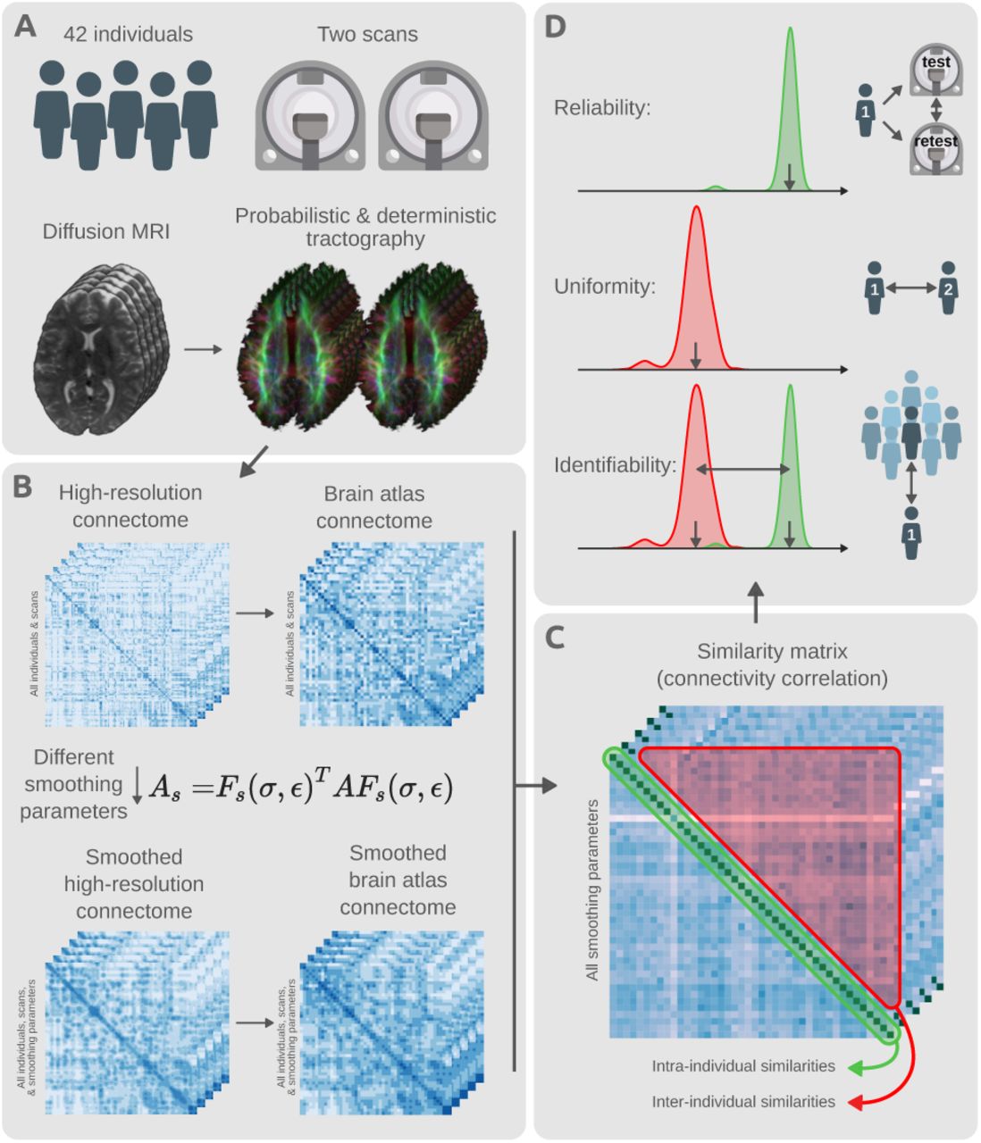
We investigated the impact of CBS on connectomes mapped at different node resolutions. As detailed below, high-resolution (60k nodes) and atlas-based (300 nodes) connectomes were mapped for individuals using diffusion MRI and established whole-brain tractography methods. Data from two diffusion MRI acquisitions for each individual were used, enabling evaluation of test-retest reliability and identifiability across different smoothing parameters. Fig. 2 provides a brief overview of the study design. We next describe the diffusion MRI acquisition, whole-brain tractography and connectome mapping procedures, smoothing parameters, and the evaluation methodology used in this study.

Schema of study design and methodology. (A) Test-retest diffusion MRI scans of 42 individuals were sourced from the Human Connectome Project. This provided a duplicate scan of every individual. Probabilistic and deterministic tractography were utilized to estimate whole-brain white matter fiber trajectories for all individuals and scans. (B) Tractography results were used to map unsmoothed structural connectomes using the high-resolution fsLR-32k surface mesh. Different smoothing parameters were used to transform the unsmoothed high-resolution connectomes into various CBS smoothed alternatives. All variants of smoothed and unsmoothed connectomes were also downsampled to connectivity maps on the HCP-MMP1.0 brain atlas comprising 360 cortical regions [44]. (C) All mapped connectomes were used to evaluate the level of similarity between connectivity maps of different scans (test and retest) for each combination of parcellation resolution and set of smoothing parameters. Both intra- and inter-individual similarities were computed for all pairs of scans. (D) The computed similarities were used to evaluate the level of connectome reliability, uniformity, and identifiability: reliability quantifies the average similarity of connectomes belonging to scans of the same individual; uniformity quantifies the average conformity of connectomes belonging to different individuals; identifiability measures the extent to which scans of the same individuals are differentiable from the rest of the group.
2.3. Imaging data acquisition and pre-processing
Imaging data were sourced from the Human Connectome Project (HCP) [39, 40]. We obtained the diffusion and structural MRI images from the 42 healthy young adults comprising the HCP test-retest cohort. For these individuals, two separate imaging sessions were conducted across two different days, with the intervening period between the test and retest scans ranging from 18 to 343 days. These duplicate individual scans enabled the assessment of both intra- and inter-individual variations in the mapped connectivity information. Diffusion MRI data were acquired using a 2D spin-echo single-shot multiband EPI sequence with a multi-band factor of 3 and monopolar diffusion sensitization. The diffusion data consisted of three shells (b-values: 1000, 2000, 3000 s/mm2) and 270 diffusion directions equally distributed within the shells, and 18 b=0 volumes, with an isotropic spatial resolution of 1.25mm [41]. We analyzed preprocessed diffusion data, where preprocessing was completed by the HCP team, using an established minimal preprocessing pipeline (v3.19.0). This included b=0 intensity normalization across scanning sessions, EPI and eddy-current-induced distortion corrections, motion correction, gradient nonlinearity correction, registration to native structural space, and masking the final data with a brain mask [42].
2.4. Connectome resolution
We mapped both high-resolution and atlas-based connectomes to evaluate the impact of CBS on different parcellation granularities. All high-resolution connectomes were mapped on the fsLR-32k standard surface mesh, comprising 32,492 vertices on each hemi-sphere [43]. This space is recommended for high-resolution cross-subject studies of diffusion MRI as it provides an accurate representation of the cortical surface with fewer vertices than the native mesh [42]. The combined left and right cortical surfaces consisted of 59,412 vertices after exclusion of the medial wall. The high-resolution maps were downsampled to a lower spatial resolution defined by the HCP-MMP1.0 atlas comprising 360 cortical regions [44]. The downsampling procedure is detailed in the Section 2.7. CBS for atlas-based connectivity. In brief, the high-resolution connectivity matrix was aggregated across all vertices belonging to each atlas region such that the connectivity weight between two atlas nodes was equal to the sum of the connectivity weights over all high-resolution vertices connecting those atlas nodes. The subcortex was not included in either high-resolution or atlas-based connectomes.
2.5. Tractography & connectome construction procedure
The impact of CBS was evaluated on both probabilistic and deterministic tractography algorithms. MR-trix3 software was used to perform tractography [45]. An unsupervised method was used to estimate the white-matter (WM), grey-matter (GM), and cerebrospinal fluid (CSF) response functions [46] for spherical deconvolution [47]. The fiber orientation distribution (FOD) in each voxel was estimated using a Multi-Shell, Multi-Tissue Constrained (MSMT) spherical deconvolution, which improves tractography at tissue interfaces [48]. The fsLR-32k surface mesh was used to generate a binary voxel mask at the interface between WM and cortical GM, from within which tractography streamlines were uniformly seeded at random coordinates from within this ribbon. Probabilistic tractography was performed by 2nd-order integration over fiber orientation distributions (iFOD2) [49]. Deterministic tractography was performed using a deterministic algorithm that utilized the estimated FOD with a Newton optimization approach to locate the orientation of the nearest FOD amplitude peak from the streamline tangent orientation (“SD_Stream”) [50]. Five million streamlines were generated for each tractography method for each scan.
A streamlines propagation mask was generated using the intersection of voxels with non-zero white matter partial volume as estimated by FSL FAST [51] and voxels with non-zero sub-cortical grey matter volume as estimated by FSL FIRST [52]. The subcortical GM was included in the propagation mask to preserve long streamlines relaying through the subcortex, only terminating streamlines at the boundaries of cortical GM or CSF. The streamline end-points were then mapped to the closest vertex of the individual’s WM surface mesh (fsLR-32k). Streamlines ending far from the cortical vertices (>2mm) were discarded. The remaining streamlines were used to generate a 59,412 × 59,412 high-resolution connectivity matrix for each of the two sessions for each individual. These data form the input for evaluation of CBS as described in the following sub-sections.
2.6. Smoothing parameters
The matrix of spatial smoothing kernels, Fs, determines the spatial distribution of smoothing weights. We use a Gaussian function to define kernel weights, G(δ), as a function of distance from the kernel center, δ, as given by:
 Where k is the dimension of the spatial kernel. The parameter σ is the standard deviation of the Gaussian distribution which determines the strength of smoothing. In this study, smoothing was applied to the cortical surface mesh (k = 2) and was quantified by the geodesic distance over the surface mesh. Despite each subject possessing the same set of vertices, the smoothing kernel was computed separately for each scan, based on the precise inter-vertex geodesic distances on the white-matter surface mesh of each individual scan.
To compare the impact of different kernel standard deviations, smoothing kernels were computed with 1, 2, 3, 4, 6, 8, and 10mm FWHM (full width at half maximum)  .
.
A second parameter that can impact smoothing is truncation of the kernel. As the Gaussian distribution decays exponentially with distance, the kernel is effectively zero for sufficiently large distances, and so contributions can be ignored with minimal loss of precision. Truncation results in a sparse smoothing kernel, enabling computationally efficient smoothing of high-resolution connectomes. Here we studied the effect of the truncation threshold, ε, which is defined as the fraction of the kernel integral discarded as a result of kernel truncation (Fig. 3A): for each value of FWHM, we generated three kernels for assessment, corresponding to ε = {0.1, 0.01, 0.001}. This truncation can alternatively be expressed as a kernel radius R (which has benefits both conceptually and programmatically):

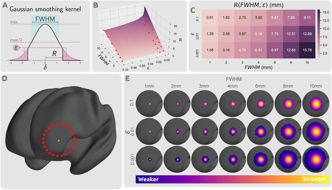
Impact of kernel parameters on truncated kernels. (A) Distribution of a truncated Gaussian kernel with smoothing parameters FWHM, ε, and R(FWHM, ε). FWHM determines the standard deviation of the Gaussian kernel, ε dictates the proportion of the kernel that is truncated, and R determines the threshold radius beyond which the kernel is set to zero. The thick black line represents the smoothing kernel as a function of the smoothing parameters. (B) Smoothing parameter space of FWHM, ε, and R. The parameter space plane shows the value of smoothing kernel radius R as a function of kernel standard deviation, FWHM, and truncation threshold, ε. The radius is linearly related with FWHM, but log-linearly with the inverse of ε. The red points indicate the selected smoothing parameters from the parameter space that were used in this study. (C) The values of kernel truncation radius at the respective smoothing parameters selected for FWHM and ε. (D) A sample cortical vertex in the left frontal lobe of an inflated cortical mesh. (E) The respective column of the smoothing kernel Fs for the vertex shown in panel (D) with different smoothing parameter choices projected on the cortical surface.
Proof of this relationship is provided in the Supplementary Information Section S.1. Thresholding radius.
Fig. 3A shows the influence of FWHM and ε on the truncated kernel. Fig. 3B,C show the relationship between standard deviation, truncation threshold and radius. Truncated kernels were generated with nonzero kernel weights only at locations with distance less than R(FWHM, ε) from the kernel center. Consequently, kernels were re-normalized such that for every vertex the column sum of Fs was 1.0 despite truncation. Fig. 3D,E demonstrate the spatial distribution of a single row of this smoothing kernel over a sample cortical surface mesh.
2.7. CBS for atlas-based connectivity
As described in Section 2.4. Connectome resolution, smoothed versions of the parcellation-based atlas-resolution connectome can be computed by first applying smoothing to the high-resolution connectome, then aggregating the connectivity values within the vertices corresponding to each atlas parcel. This approach however necessitates the high storage and computational complexity demands of high-resolution connectome data. We therefore derived a more computationally efficient procedure to perform CBS on atlas-based connectomes.
A brain parcellation atlas can be denoted by a binary p × v matrix P, where p is the number of brain regions in the atlas, such that the ith row of P is a binary mask of vertices belonging to the ith atlas region and each vertex belongs to at most one region (a “hard parcellation”). An atlas-based connectivity map Ap can be represented by the matrix multiplication Ap = PAPT : this operation reduces the v × v high-resolution connectivity A to a p × p atlas connectivity map Ap. To smooth Ap, the high-resolution connectivity matrix A can be smoothed to As and then downsampled to create the smoothed atlas connectivity map Asp. An equivalent approach is to first spatially smooth every row of the brain atlas P, and then normalize every column to produce a smoothed “soft parcellation” Ps = PFs, where each region is now defined as a weighted probability map across vertices and vertices can have non-zero membership to multiple regions. This enables direct computation of smoothed parcellation-based connectome matrix Asp without necessitating computation of the smoothed high-resolution connectome matrix As (see Supplementary Information Section S.2. CBS for atlas-based connectivity for detail):

2.8. Connectome similarity
To evaluate the potential advantages of smoothing, a measure of similarity based on Pearson’s correlation was used to quantify the conformity of two connectivity maps [32, 53]. To compute the similarity between two networks A1 and A2, first, Pearson’s correlation was computed for all respective rows of the connectivity matrices, yielding v correlation coefficients, each indicating the connectivity similarity of a single node; these correlations were then averaged over all nodes to produce a single value indicating the similarity of two connectomes. This measure was used to quantify both intra- and inter-individual connectome matrix similarities.
2.9. Evaluation metrics
Direct connectome comparisons were performed within each combination of: tractography algorithm (deterministic and probabilistic); parcellation resolution; and network smoothing parameters. Within each of these configurations, smoothed structural connectomes were generated independently for the two scanning sessions for each of 42 participants. For each scan in session 1, its similarity to every session 2 scan (1 intra-individual and 41 inter-individual) was computed; aggregated across all individuals, this process yielded 42 values comparing connectomes of the same individual (intra-individual similarities), and 42 × 41 measuring the similarity between connectomes of different individuals (inter-individual similarities). The intra-individual similarities were averaged to form a measure of connectome reliability µintra, indicating the extent of consistency of mapped connectomes for an individual; similarly, the inter-individual similarities were averaged to yield a measure of population uniformity of the connectivity maps µinter. Ideally, connectomes should be reliable (i.e. high µintra) and preserve inter-individual differences (i.e. low µinter). Hence, high reliability and low population uniformity is desirable.
To evaluate the extent to which an individual’s connectome is unique, we adopted an established identifiability framework [54]. Identifiability quantifies the extent to which an individual can be differentiated from a larger group based on a set of individual attributes. Here, identifiability was measured by the effect size of the difference in the means of intra-individual and inter-individual similarities [32]:
 Where µintra and µinter are the mean of the two intra- and inter-individual similarity distributions and s is the pooled standard deviation of the two distributions.
2.10. Evaluating statistical power with atlas-resolution smoothing
Generally, smoothing can result in a loss of effective spatial resolution, blurring, and shifting or merging of adjacent signal peaks [55–58], but is necessary to strike a compromise between sensitivity and specificity [59]. Hence, we investigated the impact of CBS on mass univariate significance testing of associations between cognitive performance and atlas-based structural connectivity. Given that structural connectivity and cognition are known to be associated [32], we tested whether the use of CBS would improve power to detect such associations. For each pair of regions in the parcellation atlas, Pearson’s correlation coefficient was used to test for an association between connectivity strength and a previously established measure of overall cognitive performance [60]. This yielded a correlation coefficient for each pair of regions. Age and sex were regressed out from the cognitive measure as confounds. This was repeated across 100 bootstrap tests each including 90% of the sample (N=35) to increase the robustness of the comparisons against individual effects.
To generate a distribution of correlation coefficients under the null hypothesis of an absence of association between connectivity and cognitive performance, we randomized cognitive scores between individuals and recomputed all correlation coefficients; this was repeated for 1000 randomizations (10 randomizations within each bootstrap sample), yielding 1000 correlation coefficients representing the null distribution for each connection. For a range of correlation coefficient thresholds from 0.1 to 0.5 (which indicate small to large effects according to Cohen’s conventions [61]), we counted the number of suprathreshold connections in both the empirical and randomized data (averaged across the 1,000 randomizations).
From these data, we generated an ROC (Receiver Operator Characteristic) curve as follows. The number of suprathreshold connections in the empirical data was assumed to give the combined number of true positives (TP) and false positives (FP), while the average total number of suprathreshold connections in the randomized data estimated the total number of FP (Fig. 4A). The combined number of false negatives (FN) and true negatives (TN) was determined by subtracting TP +FP from the total number of connections. Finally, since the true underlying effect was unknown, we assumed a false omission rate of 1%, i,e.,  . This assumption enabled estimation of sensitivity
  and specificity
  that were used to generate the ROC curve. We ensured that our estimates were robust to the choice of λ (see Supplementary Information Section S.3. Replication of ROC curve estimates for detail). This process was repeated independently for various smoothing kernels, and for data generated using both deterministic and probabilistic tractography algorithms, to investigate the impact of CBS on the statistical power to detect associations between cognitive performance and connectivity.

Estimation of receiver operating characteristic (ROC) curves for mass univariate testing of associations between cognitive performance and structural connectivity. For each pair of regions in the parcellation atlas, Pearson’s correlation coefficient was used to test for an association between connectivity strength and a previously established measure of overall cognitive performance. (A) For a given effect size threshold (horizontal axis), the number of suprathreshold connections (vertical axis) yielded the combined number of true positives (TP) and false positives (FP), indicated by the green line. The red line indicates the total number of FP, determined by randomizing cognitive scores between individuals and recomputing all correlation coefficients (1000 randomizations; mean & 95% confidence interval shown). (B) Assuming a constant value for the false omission rate  , an ROC curve can be estimated for different effect size (correlation coefficient) thresholds. TPR: true positive rate. FPR: false positive rate.
Additionally, we tested the replicability of the suprathreshold effects in a test-retest comparison to evaluate the replicability of the observations before and after smoothing. At each utilized threshold value, for every edge that was suprathreshold in the data from either session 1 or session 2, we calculated the difference in correlation coefficient between the two sessions. This provided a distribution of effect differences observed across a range of effect thresholds. Thus, a lower average effect difference indicated higher consistency of the connectivity-behavior observations and higher replicability of the findings.
3. Results
We investigated the utility of CBS for high-resolution and atlas-based connectomes, focusing on connectome reliability and identifiability as well as computational and storage requirements. We recommend optimal smoothing kernels for connectomes mapped with deterministic and probabilistic tractography, and we demonstrate that smoothing improves the statistical power to detect associations between connectivity and cognitive performance.
3.1. High-resolution connectome storage size
High-resolution connectomes require considerable storage and computational resources, and CBS can increase this burden, due to reductions in matrix sparsity. Fig. 5 summarizes the sizes of stored connectomes for various kernels. Kernels with larger FWHM and/or more lenient truncation thresholds incur greater storage demands for high-resolution connectomes. We found that the kernel radius R(FWHM, ε), which is dependent on both parameters, was a reasonable predictor of connectome size. We also observed that connectomes mapped using probabilistic tractography were approximately an order of magnitude larger than their deterministic counterparts both prior to smoothing (10MB for probabilistic and 1MB for deterministic) and after performing CBS with identical smoothing parameters.

Impact of CBS on connectome storage requirements. (A) Tables show the mean storage size of individual connectomes mapped using deterministic (upper) and probabilistic (lower) tractography following smoothing, as a function of truncation threshold and full-width at half maximum (FWHM) of smoothing kernel (B) The relationship between the kernel radius and file size of individual connectomes. Results for connectomes with no smoothing are marked with an x. File sizes are plotted using a logarithmic scale. Shaded bands indicate one standard deviation from the mean.
3.2. Identifiability and reliability
Fig. 6 summarizes the impact of CBS on the identifiability and reliability of high-resolution structural connectivity maps. We observed that both larger FWHM values and smaller truncation thresholds (i.e., larger R in both cases) consistently improved connectome reliability (mean intra-subject similarity). While high-resolution connectomes without smoothing had a relatively low reliability (µintra < 0.2), CBS with kernels as little as 3-4mm FWHM resulted in a substantial increase in reliability (µintra > 0.5), with reliability exceeding 90% (µintra > 0.9) achieved in some scenarios.

Impact of CBS on high-resolution connectomes for a range of different kernel parameters. Reliability (first row) and identifiability (second row) are reported for deterministic (left column) and probabilistic (right column) structural connectomes mapped at the resolution of cortical vertices. Results for connectomes with no smoothing are marked with an x in each plot. Kernel truncation thresholds, ε, are colored using warm colors such that each line connects points with equal ε; similarly, FWHM is colored using shades of green.
CBS also impacted connectome identifiability. We observed that while CBS with a 2-4mm FWHM kernel improved the identifiability of connectomes, CBS with larger FWHM was detrimental for individual identifiability, such that CBS with a 10mm FWHM resulted in more than 50% reduction in identifiability. For both identifiability and reliability measures, CBS was more sensitive to a change in kernel FWHM in contrast to the truncation threshold ε. Increasing the truncation threshold from ε = 0.01 to ε = 0.001 had negligible impact on either measure.
Tractography algorithm choice also impacted reliability and identifiability. High-resolution connectomes mapped using deterministic tractography had relatively lower reliability (10-20% lower), but higher identifiability (20-30%), compared to their probabilistic counterparts with identical CBS parameters.
Fig. 7 shows the impacts of CBS with different kernel parameters on an atlas-parcellation-based structural connectome. In agreement with the high-resolution analyses, we observed both that increases in FHWM and decreases in kernel truncation thresholds led to improved connectome reliability, and that this improvement in reliability comes at the expense of reduced identifiability. Without CBS, the atlas-based connectomes were already relatively reliable (deterministic: 92%, probabilistic: 98%). Use of the largest smoothing kernel increased these to 97% and 99%, respectively, albeit at the cost of a small reduction in identifiability (from 7.8 to 7.2 for deterministic and from 6.8 to 6.1 for probabilistic). Changing kernel extent from ε = 0.01 to ε = 0.001 again had no considerable impact on reliability or identifiability. The magnitude of influence of CBS on the atlas-resolution connectomes was comparatively smaller than the effects observed at the higher resolution.

Impact of CBS on atlas-based connectomes, for a range of different kernel parameters. The connectome reliability (first row) and identifiability (second row) are reported for deterministic (left column) and probabilistic (right column) structural connectomes mapped at the resolution of atlas parcels. The unsmoothed atlas-based connectivity results are marked with x in each plot. Kernel truncation thresholds, ε, are colored using warm colors such that each line connects points with equal ε; similarly FWHM is colored using shades of green.
All in all, we observed that the advantages of CBS for high-resolution were maximized with 3-6mm FWHM kernels; larger smoothing kernels (>6mm FWHM) could deteriorate high-resolution identifiability for the sake of reliability. In contrast, identifiability of the atlas-resolution maps were less sensitive to larger smoothing kernels, and thus kernels of 6-10mm FWHM can be used to improve reliability with proportionally smaller losses in identifiability. To achieve similar reliability and identifiability, connectomes generated using deterministic tractography were found to require CBS with larger smoothing kernels compared to their probabilistic counterparts.
Finally, it should be noted that the optimal CBS kernel parameters essentially depend on the application for which the connectome will be used.
3.2.1. Case Study: Impact of CBS on statistical power
Finally, we investigated whether CBS can improve statistical power to detect associations between structural connectivity and cognitive performance. For this study we used FWHM = 8mm and ε = 0.01, based on the results reported above. For this case study, we considered the mapped atlas-based connectomes and computed Pearson’s correlation coefficient between streamline counts and cognitive performance for each pair of regions. ROC curves were then computed for each case, as described in the Methods, to determine whether CBS improved statistical power to identify associations between connectivity and cognitive performance.
First, we tested whether the magnitude of effect in the set of suprathreshold connections (i.e., connections with a correlation coefficient exceeding a fixed threshold) were replicable between the test and retest datasets. We found that CBS improved replicability in suprathreshold connections, particularly more so for connectomes mapped with probabilistic tractography (Fig. 8A); this suggests that CBS can improve the reproducibility of mass univariate testing on connectomes.

Impact of CBS on statistical power of mass univariate testing on atlas-based connectomes, based on an exemplar dataset examining correlations between structural connectivity and cognitive performance. (A) Replicability of suprathreshold connections between test and retest datasets: a lower difference of the observed effect magnitude between test and retest is favorable in terms of replicability. (B) The number of suprathreshold connections as a function of the effect size threshold was compared with a null distribution from permutation. To assess the predictive utility of the connectomes, precision, sensitivity, and specificity was estimated from a comparison with the null. (C) Precision was calculated from the ratio of supra-threshold edges found in empirical data compared to the null model at different effect thresholds. (D) ROC curves were estimated to demonstrate the respective changes in sensitivity  and specificity
  of the edges selected at different effect thresholds. The analyses were repeated across bootstrap samples to provide a robust estimate of statistical power. Shaded lines indicate 95% confidence intervals. Abbreviations: TP: True Positive, FP: False Positive, TN: True Negative, FN: False Negative, TPR: True Positive Rate, FPR: False Positive Rate.
Next, we enumerated the number of suprathreshold connections as a function of the effect threshold (Fig. 8B). While the proportion of suprathreshold connections increases following smoothing for the empirical data, indicating a potential gain in sensitivity, a similar increase in the randomized (null distribution) data suggests that this may come at the expense of poorer specificity. For connectomes mapped with deterministic tractography, the numbers of suprathreshold connections for the empirical and randomized data are separated by a comparable gap, irrespective of whether CBS was performed. For probabilistic tractography, the number of suprathreshold connections for the randomized data was comparable with and without smoothing, whereas CBS resulted in a substantially greater proportion of suprathreshold connections for the empirical data. This suggests that CBS can improve the statistical power of mass univariate testing performed on connectomes mapped with probabilistic tractography, without a substantial loss in specificity.
To further investigate these effects, we considered precision  as a function of effect size threshold (Fig. 8C); and from this, generated ROC curves (Fig. 8D). Performing CBS on connectomes mapped from probabilistic tractography improves the precision and sensitivity of the inference. This improvement is also partially observed for connectomes mapped from deterministic tractography only for smaller effect thresholds (r < 0.3). Taken together, these results suggest that CBS is particularly beneficial to improving the statistical power of inference performed on connectomes mapped with probabilistic tractography; in contrast, for connectomes mapped with deterministic tractography, the benefit of CBS is marginal and possibly detrimental for larger effect size thresholds (r > 0.3). More importantly, CBS improved replicability with minimal impact on the statistical power for connectomes mapped with both tractography algorithms.
4. Discussion
In this study, we established a computationally efficient formalism for connectome smoothing and demonstrated that our connectome-based smoothing (CBS) method can benefit the analysis of atlas-based and high-resolution connectomes. Our results demonstrate that CBS impacts different aspects of connectivity mapping analyses, including individual reliability, inter-individual variability, and the interscan replicability of brain-behavior statistical associations, as well as computational storage demands. The choice of smoothing kernel parameters involves a trade-off between connectome sensitivity and specificity: larger kernels (higher FWHM and lower ε) improve connectome sensitivity, but are detrimental to connectome specificity. It is therefore important to select a level of smoothing that strikes a balance between these competing factors. In the following sections, we provide some guidelines for selecting optimal smoothing parameters and discuss the implications of performing CBS for connectome reliability, identifiability, storage requirements, and statistical power.
4.1. Appropriate smoothing parameters
Our results indicate that CBS differentially affects the characteristics of structural connectivity matrices mapped with different tractography methods and parcellation resolutions. Although we cannot suggest a one-size-fits-all smoothing kernel, our findings can guide selection of appropriate CBS smoothing kernels in future studies. Table 1 provides some rules of thumb for selecting a level of spatial smoothing which aims to achieve a balance between reliability and identifiability, while also considering storage demands. In general, high-resolution connectomes benefit from smaller FWHM compared to atlas-based connectomes, and deterministic maps require larger FWHM than their probabilistic counterparts to achieve the same level of reliability. However, the goals of the analysis at hand must be considered when selecting the level of smoothing. For example, if the goal is to identify an individual from a group based on their connectome, deterministic tractography and a smaller FWHM than recommended in Table 1 may be desirable. On the other hand, if one wishes to build a reliable consensus structural connectome that is robustly consistent across individuals, a higher FWHM than recommended in Table 1 may be favored. A value of 0.01 is suggested universally for the kernel truncation threshold ε, as smaller thresholds yield negligible impacts on identifiability and reliability whilst incurring much greater storage costs.
Recommended smoothing parameters. This table provides rule of thumb recommendations for CBS smoothing kernels of different variants of structural connectomes. In general, connectomes at the resolution of a brain atlas can benefit from larger CBS kernels compared to high-resolution connectomes. High-resolution connectomes computed from probabilistic tractography are advised to be smoothed less than their deterministic counterparts. Reducing epsilon below 0.01 is unfavorable and computationally costly. The rounded values for kernel radius R(FWHM, ε) provide sensible approximations.
Without CBS, connectomes mapped from deterministic tractography were found to yield higher identifiability; conversely, connectomes mapped from probabilistic tractography were more reliable. This is in line with previous reports suggesting that probabilistic tractography achieves higher sensitivity, lower specificity, and lower interindividual variability, compared to deterministic approaches [62–65]. Given that many factors other than reliability and identifiability would affect the choice of tractography algorithm, we suggest that CBS could be leveraged to achieve a balance between reliability and identifiability of the selected tractography algorithm. Hence, we could take advantage of a comparatively larger kernel for deterministic tractography approaches to match the reliability and identifiability of the probabilistic counterpart.
Our results highlight that CBS is a critical step to improving the reliability of high-resolution connectomes. High-resolution connectivity mapping is particularly sensitive to noise, artefacts, and registration misalignment, all of which can be alleviated—to a certain extent—with the new CBS formalism developed here.
4.2. Connectome reliability
Structural connectivity maps are commonly used in research to draw statistical inferences regarding associations between brain connectivity and different aspects of human cognition, behavior, and mental health [66–71]. The statistical power of such inferences can depend on the reliability of the measure under study: a connectivity measure that can be reliably assessed for all individuals can potentially improve the characterization of brain-behavior associations. However, improvements in reliability achieved by increasing the level of smoothing come at the expense of poorer spatial specificity and increases in connectome storage and computational requirements. CBS enables researchers to balance this trade-off to match the goals of the analysis at hand. Commonly used atlas-based connectivity maps are comparatively reliable, even without any smoothing, since the reduced spatial resolution of inter-subject correspondence imposed by a parcellation performs an operation comparable to smoothing. Nevertheless, we found that CBS could marginally improve the reliability of atlas-based connectomes.
4.3. Individual identifiability
The concept of neural fingerprinting has emerged in recent years which considers the challenge of identifying an individual from within a large group of others, based on their connectome or other neuroimaging data [53]. While the efficacy of a measure at individual identification does not necessitate existence of behavioral and pathological biomarkers in individuals, it could still be conceived as an indicator of the strength of such individual brain-behavior associations. By reducing the impact of noise and registration misalignments, CBS can enhance detection of individual differences in connectivity maps, enabling clearer differentiation of individuals and thus potentially improve the accuracy of neural fingerprinting. Our findings suggest that a minimal smoothing kernel of 2mm FWHM improves both reliability and identifiability of high-resolution connectivity matrices. Implementing CBS with larger kernels (i.e. > 2mm FWHM) further enhances connectome reliability substantially, but results in a gradual reduction in identifiability due to loss of individual identifiers by spatial blurring. Smoothing the high-resolution connectivity maps beyond 6mm FWHM is unnecessary because gains in reliability diminish, despite detrimental impacts on identifiability, spatial specificity, and storage requirements.
4.4. Storage requirements
It is important to consider the storage demands and associated computational burdens of handling smoothed connectome data. If the connectome size is larger than a gigabyte or so, handling the file (loading into memory and conducting analyses) can become unacceptably time-consuming. Even with the assistance of high-performance computing infrastructure, any benefits of using connectomes larger than a few gigabytes might not outweigh the time and resources required to process the larger files. This especially limits the extent of smoothing for connectomes generated using probabilistic tractography, which can grow to more than a few gigabytes when smoothed above 4-6mm FWHM. In contrast, connectomes mapped with deterministic tractography can be smoothed further whilst remaining highly computationally feasible. Nevertheless, if greater smoothing is essential in a study, a high-performance computing platform with access to adequate memory can be used to process smoothed connectomes (potentially without use of sparse matrix data structures), which may take tens of gigabytes of memory per individual connectome.
4.5. Implications on atlas resolution
Our results highlight the impact of CBS on structural connectomes mapped both at the high resolution of individual surface vertices, and the lower resolution of a brain atlas. While the findings vary in terms of magnitude of influence, a common pattern is visible across resolutions: higher FWHM results in a more reliable connectome, yet higher FWHM reduces the identifiability of connectomes. We developed computationally efficient methods to perform CBS at both resolutions. Atlas-based connectivity matrices have a relatively small memory footprint (<1MB), and thus they can be processed and stored efficiently, regardless of the level of smoothing. Similar to the high-resolution connectomes, when using an atlas parcellation, probabilistic and deterministic tractography approaches have complementary attributes when comparing reliability and identifiability: connectomes mapped from probabilistic tractography achieve better reliability compared to their deterministic counterparts, whereas deterministic connectomes can better reveal individual differences. This is one possible factor that can guide the choice between deterministic and probabilistic tractography algorithms. However, CBS can be used to increase the reliability of connectomes mapped from deterministic tractography to match the reliability of the probabilistic approach.
Finally, the atlas-based smoothing results suggest that probabilistic maps are to a certain extent representative of highly smoothed deterministic ones. In other words, more smoothed deterministic maps were analogous to less smoothed probabilistic maps, as the probabilistic evaluation curves in Fig. 7 seem to be a continuation of the deterministic curves. This observation is in agreement with prior expectations given the mechanisms used to generate the data, as probabilistic tractography-based connectivity has an intrinsic spatial smoothness due to the stochastic variability in streamline propagation. The proposed method to perform CBS on atlas-based connectomes does not require construction of any intermediate high-resolution connectomes and is a fast operation relative to the time required to perform whole-brain tractography. Thus, while the benefits of spatial smoothing for atlas-based connectomes were modest, we recommend including CBS in future connectome mapping workflows.
4.6. CBS and principals of spatial smoothing
Our proposed connectome-based spatial smoothing approach is an extension of spatial signal smoothing to networks, and hence, fundamental concepts within the domain of spatial smoothing are applicable to CBS. For instance, from a signal processing perspective, the matched filter theorem states that spatial smoothing by an appropriate Gaussian kernel equalizes the voxel-wise standard deviation and, in turn, yields an optimal sensitivity to detect effects of unknown extent [72, 73]. Additionally, with regards to single-subject inference, such smoothing facilitates the application of multiple comparison correction using random field theory [72–74] and finally, smoothing mitigates residual anatomical variability of individuals at the group-level. These concepts are equally applicable to CBS, wherein, a matrix multiplication with a smoothing kernel achieves a similar purpose to convolution of image data with a 3D spatial smoothing kernel; as a result, CBS can be utilized to (i) maximize connectivity SNR through appropriate filter selection, (ii) improve single-subject inference, and (iii) improve the reliability of group level connectivity analyses. This poses an interesting future research direction to explore the benefits of CBS for whole-brain high-resolution network inference in which voxel-wise approaches [31, 74–76] are combined with network-based approaches [30].
4.7. Concluding remarks
In this study, we developed a novel formalism for connectome-based smoothing of structural connectivity matrices and demonstrated the wide-ranging benefits of connectome smoothing. Our results indicate that CBS with different kernel FWHMs and truncation thresholds significantly impacts various characteristics of structural connectivity matrices. In high-resolution connectomes, smoothing up to 3-6mm FWHM was deemed favorable, though the choice of smoothing parameters imposes a trade-off between reliability and individual identifiability. We provided recommendations for smoothing parameter choices that achieve a compromise between reliability and identifiability. Our connectome-based smoothing method and associated recommendations can be incorporated into future structural connectivity mapping pipelines, enabling more reliable and better powered connectome analyses. Moreover, high-resolution structural connectivity overcomes the known uncertainty and ambiguity in determination of brain parcellation, and so will be a powerful analysis framework moving forward; our demonstrated and evaluated smoothing framework is an essential tool in facilitating such, and we have made reasonable recommendations for how others can use it.
Data and code availability
All imaging data used in this study was sourced from the Human Connectome Project (HCP) (www.humanconnectome.org). The bash scripts used to perform tractography using MRtrix3 [45] (www.mrtrix.org), as well as all Python code required to perform CBS and map smoothed connectomes at either the resolution of vertices or an atlas, are provided in our git repository. This code repository can be accessed from github.com/sina-mansour/connectome-based-smoothing. Additionally, to facilitate future research, the codes for smoothing connectomes at high-resolution and atlas-resolution will be released as a standalone python package (currently under development).
Author contributions
S.M.L.: Conceptualization, Methodology, Formal analysis, Data curation, Software, Writing - original draft, Writing - review & editing C.S.: Conceptualization, Writing - original draft, Writing - review & editing R.S: Conceptualization, Writing - original draft, Writing - review & editing A.Z: Supervision, Conceptualization, Writing - original draft, Writing - review & editing
Competing interests
The authors declare no competing interests.
Supplementary Information
S.1. Thresholding radius
This section provides the mathematical rationale behind the relationship between R, σ (or alternatively FWHM), and ε presented in Equation 6. The truncation radius R was formulated as a function of σ and ε such that the proportion of signal loss for a 2-dimensional Gaussian kernel with the strength of σ truncated at a radius of R is equal to ε. Given that the Gaussian kernel was defined such that its total cumulative density is unity  , the relationship between the smoothing parameters can be defined by the following integration over the 2-dimensional surface area:
 This integration can be solved in polar coordinates by the following closed form equation:
 And this can be used to describe R as a function of σ and ϵ:
 And given the relationship between FWHM and
  , this equation can be rewritten based on FWHM:

S.2. CBS for atlas-based connectivity
In the main text, it was briefly mentioned that mapping the high-resolution connectivity is not necessary for smoothing the connectivity matrices at an atlas resolution: alternatively, a smoothed version of an atlas-based connectivity matrix can be derived from a soft parcellation, which is derived by applying spatial smoothing to the parcels of the brain atlas (and normalizing each vertex to a unity sum of parcel memberships). In this section, we provide the formal proof of this equivalence: first, downsampling a high-resolution connectivity matrix to an atlas-based connectome matrix is formulated by linear algebraic formulations; these formulations are then used to complete a formal proof of the equivalence.
Following the prior nomenclature, A is a v × v matrix denoting the high-resolution connectivity matrix where v is the number of vertices. According to Equation 4, the smoothed high-resolution connectivity matrix As is calculated as follows:
 Where Fs is a v × v column-normalized spatial smoothing kernel. A formal notion of a brain atlas can be denoted by p × v matrix P, where p is the number of brain regions in the atlas. Elements P (i, j) encode the relationship between vertex/voxel vi and region pj.
 An atlas-resolution connectome Ap is a p × p matrix, which is normally mapped from an atlas parcellation such that elements Ap(i, j) encode the aggregate contribution from those streamlines for which one endpoint is assigned to region pi and the other endpoint is assigned to region pj (showing here the streamline count for simplicity):
 This notion can be formalized by the following matrix representation which can be used to derive Ap from A and P :
 Hence, the element Ap(i, j) counts the overall connectivity between regions pi and pj by adding all high-resolution connectivity edges between them. Equations S5 and S8 yield the following definition for the smoothed atlas-based connectivity Asp:
 The matrix PFs can thus be treated as a p × v weighted soft parcellation map, i.e. a non-binary brain atlas. This soft parcellation can be used to generate smoothed connectomes based on an atlas parcellation (each streamline contributes to many connectome edges, based on all parcels with non-zero densities at both end-points) (see Equation S8). A key benefit of this approach is that it obviates the need to create computationally cumbersome high-resolution connectomes as an intermediate step in construction of lower-resolution connectome matrices. A different approach to compute this soft parcellation, that additionally does not necessitate computation of high-resolution smoothing matrix Fs, is further described in the ensuing sections.
S.2.1. Column normalization
To describe the soft parcellation PFs, a formal definition of normalizing every column should first be defined. Column normalization of an l × m matrix B can be defined by the matrix multiplication of B with a diagonal norm matrix constructed from column sums.
⟨|B|⟩ denotes an m m diagonal column norm matrix constructed from B where ⟨|B|⟩ (i, i) is the sum of the elements of the ith column in B:
 Hence,
 And a consequence of Definition S.1 is the statement in the next corollary.
Let zi ∈ ℝi denote the vector of ones, i.e. all i vector elements equal 1. The following is true for any diagonal norm matrix:
 Both sides of the equation above compute the column sums of B. Column normalization can be formally defined by the following theorem.
The row normalization is a matrix transformation of an l × m matrix B to an l m normalized matrix N (B), such that the sum of every column in N (B) is equal to 1, i.e. zlN (B) = zm. N (B) can be derived by the following matrix multiplication:
 Proof. Corollary S.1.1 can be used to prove zlN (B) = zm:
 □
□
Where Im is the m × m identity matrix. The following remarks are a consequence of the aforementioned definitions and theorems.
Remark. The diagonal norm matrix of a brain atlas parcellation ⟨|P|⟩ is the v × v identity matrix Iv, as every vertex belongs to a single atlas region and thus the sum of any column of P equals 1:
 Thus, for any arbitrary v × v matrix X:
 ⟨|PX|⟩, by definition, is a diagonal matrix:
 and from Equation S14 we know that:
 Therefore, ⟨|X|⟩ is the same diagonal matrix as PX. In other words, the sum of the columns of PX is equal to the sum of the columns of X.
Remark. The normalized high-resolution smoothing kernel Fs is defined from column normalization of the Gaussian kernel smoothing weights matrix FG (from Equation S13):
 Where FG is a symmetric v × v matrix yielded from the truncated Gaussian function calculated upon the surface mesh:

S.2.2. Smoothed brain atlas
Equation S9 showed that a smoothed soft parcellation Ps = PFs can be used to directly derive smoothed atlas connectivity maps from tractography. In this section, a formal proof will be provided for the following statement:
The smoothed soft parcellation Ps = PFs can be computed in the absence of Fs, by separately smoothing every row of P, followed by normalizing every column of the smoothed parcellation:
 Proof. Using the previously derived equations, we prove that Ps = N (PFG):
 □
□
The proof above confirms that structural connectivity based on a parcellation atlas, incorporating CBS, can be constructed directly from a tractogram and soft parcellation, without necessitating computation of either the high-resolution smoothing matrix or the high-resolution connectome. To smooth an atlas-resolution connectome, the brain atlas P should first be transformed to a normalized smoothed soft parcellation Ps = N (PFG). PFG is equivalent to independently smoothing the binary representation of each parcel, while the normalization of such ensures that the sum of parcel memberships of every vertex is 1. Hence, the soft-parcellation Ps can be computed by spatial smoothing and then be directly combined with the tractogram to produce a connectome: each streamline endpoint may have non-zero attribution to multiple parcels, and the contribution of the streamline to the connectome is therefore distributed across the set of edges associated with those two sets of parcels. This constitutes an approach to apply CBS on atlas-resolution connectomes that does not require any high-resolution connectomic computations.
S.3. Replication of ROC curve estimates
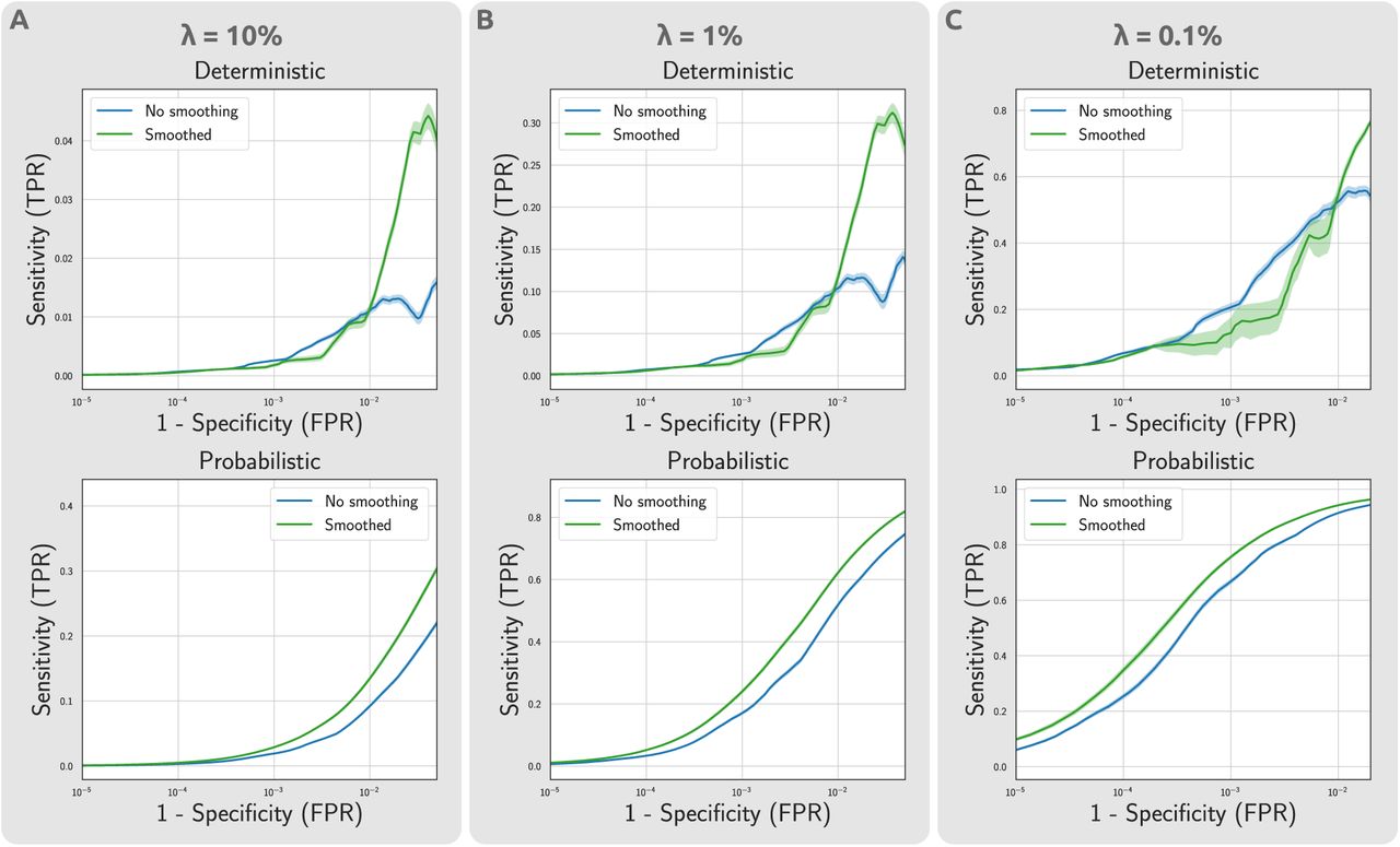
The computation of ROC curves reported in the manuscript relied on the assumption of a fixed false omission rate  . To ensure that the findings were not biased by the selected value for λ, the same analyses was repeated for a range of plausible values of λ ∈ {10%, 1%, 0.1%}. Fig. S1 presents the results of this evaluation. The findings indicate that CBS increases the sensitivity of the statistical analyses and the inference power, particularly for connectomes mapped from probabilistic tractography, regardless of the selection made for the false omission rate λ.

Impact of CBS on statistical power of mass univariate testing on atlas-based connectomes, for different false omission rate assumptions. The estimated ROC curves demonstrate the respective changes in sensitivity and specificity of the suprathreshold edges at different effect thresholds. The analyses was repeated across a range of false omission rates to ensure the robustness of findings with regards to parameter selection.
Acknowledgments
Data were provided by the Human Connectome Project, WU-Minn Consortium (Principal Investigators: David Van Essen and Kamil Ugurbil; 1U54MH091657) funded by the 16 NIH Institutes and Centers that support the NIH Blueprint for Neuroscience Research; and by the McDonnell Center for Systems Neuroscience at Washington University. The data analysis was supported by SPAR-TAN High Performance Computing System at the University of Melbourne [77], and also supported by use of the Melbourne Research Cloud (MRC) providing Infrastructure-as-a-Service (IaaS) cloud computing to the University of Melbourne researchers through the NeCTAR Research Cloud, a collaborative Australian research platform supported by the National Collaborative Research Infrastructure Strategy. S.M.L. is funded by a Melbourne Research Scholarship. R.S. is supported by fellowship funding from the National Imaging Facility (NIF), an Australian Government National Collaborative Research Infrastructure Strategy (NCRIS) capability. A.Z. was supported by a senior research fellowship from the NHMRC (APP1118153).


