

Abstract
A central challenge of medical imaging studies is to extract biomarkers that characterize pathology or predict disease outcomes. State-of-the-art automated approaches to identify these biomarkers in high-resolution, high-quality magnetic resonance images have performed well. However, such methods may not translate to low resolution, lower quality images acquired on MRI scanners with lower magnetic field strength. In low-resource settings where low-field scanners are more common and there is a shortage of available radiologists to manually interpret MRI scans, it is therefore essential to develop automated methods that can augment or replace manual interpretation while accommodating reduced image quality. Motivated by a project in which a cohort of children with cerebral malaria were imaged using 0.35 Tesla MRI to evaluate the degree of diffuse brain swelling, we introduce a fully automated framework to translate radiological diagnostic criteria into image-based biomarkers. We integrate multi-atlas label fusion, which leverages high-resolution images from another sample as prior spatial information, with parametric Gaussian hidden Markov models based on image intensities, to create a robust method for determining ventricular cerebrospinal fluid volume. We further propose normalized image intensity and texture measurements to determine the loss of gray-to-white matter tissue differentiation and sulcal effacement. These integrated biomarkers are found to have excellent classification performance for determining severe cerebral edema due to cerebral malaria.
1. Introduction
Malaria is a parasitic infection that results in more than 400,000 deaths annually, with the great majority occurring in children living in sub-Saharan Africa, and continues to be a public health priority (World Health Organization, 2018). Cerebral malaria (CM) is a serious complication of malaria infection characterized by impaired consciousness and ultimately coma (Idro et al., 2010). In children, CM is a leading cause of malarial death and has a case fatality rate of 15-20% despite optimal treatment (Dondorp et al., 2010). The pathophysiological mechanisms behind CM are not completely understood, though diffuse brain swelling, intracranial hypertension, and higher brain weight-for-age are commonly seen in fatal cases (Idro et al., 2010; Seydel et al., 2015). It is thus hypothesized that brain swelling, in conjunction with non-central nervous systemic factors, plays a critical role in disease outcome and mortality risk in particular. For this reason, brain magnetic resonance imaging (MRI) has been proposed to study the pathogenesis of CM (Looareesuwan et al., 2009) and assess participants’ eligibility for enrollment in clinical trials (Kampondeni et al., 2018). In the latter case, the severity of brain swelling (cerebral edema) must be evaluated rapidly with MRI, ideally by a trained on-call neuroradiologist.
MRI is a non-invasive technique that equips powerful electromagnetic fields to visualize brain structures and assess both disease diagnosis and prognosis. Recent trends in MRI hardware, including magnets with increasing field strengths of up to 7 Tesla (7T), have allowed us to capture extremely detailed images of the human brain. Alongside this improvement in technology, there has been a concurrent explosion of sophisticated and automated methods ranging from lesion segmentation in multiple sclerosis (Shiee et al., 2010; Valcarcel et al., 2018; Valverde et al., 2017) or brain tumor (Gordillo, Montseny and Sobrevilla, 2013), to the prediction of clinical outcomes in patients with psychosis (Nieuwenhuis et al., 2017). However, access to advanced MRI technology is not consistent across the globe (Marques, Simonis and Webb, 2019): in low-resource settings, challenges related to cost, infrastructure, and unreliable power sources may limit the availability of high field strength MRI (Latourette et al., 2010), sparking interest in lower field strength (≤ 0.5T) alternatives. Compared to high-field MRI, low-field MRI tends to produce images with lower spatial resolution. This is because signal-to-noise ratio (SNR) scales with magnet strength, and SNR is a trade-off between spatial resolution and the length of scan (Sarracanie and Salameh, 2020). Despite these challenges, low-field neuroimaging has offered diagnostic value in situations where only moderate resolution is required for a clinical assessment, such as stroke (Bhat et al., 2020), infant hydrocephalus (Obungoloch et al., 2018), and cerebral malaria (Kampondeni et al., 2013).
The field of quantitative methods that are both fully automated and that also accommodate low-field MRI scans is currently understudied. Automated methods are of particular relevance to resource-limited settings, because there is often a shortage of available radiologists that can manually interpret brain scans, even when MRI is available. In the context of a current clinical trial in CM, rapid interpretation of brain MRI scans is needed at all hours of the day to determine whether affected children might benefit from more aggressive treatment, which has required off-shore radiologists in different time zones to volunteer their time. Moreover, as visual determinations are typically unstructured and involve a degree of subjectivity, there is growing demand for radiographic data that can be captured as a quantitative assessment (Potchen et al., 2013). An open question is whether modern image analysis pipelines—which were developed on higher resolution images—can be translated to low-resolution and lower quality scans, and thereby provide valuable clinical information from a brain MRI even in low-resource settings.
In this paper, we first address this question by experimenting with a common pre-processing task in brain MRI analysis referred to as brain segmentation, where 3-dimensional pixels (voxels) of the brain are identified and isolated from other voxels in the image. We show that popular surface-based methods such as the Brain Extraction Tool (Smith, 2002) perform well on 3T images, but poorly on the 0.35T images in our sample (Figure 1), despite parameter tuning. We then present a novel, integrative framework that adapts image processing pipelines originally designed for high field strength scanners to images from low field strength scanners. We demonstrate that existing high-quality brain imaging data can be leveraged to identify cerebral tissue and remove all non-brain voxels from lower-quality images. We then adapt currently available image processing techniques to extract volume-, intensity-, and curvature-based biomarkers from low resolution MRI scans. This approach is applied to images acquired on a 0.35T scanner to assess the severity of cerebral edema in children with CM. To parsimoniously assess each of the radiographic criteria used in manual assessments, we incorporate the derived imaging biomarkers into a logistic regression model to predict severely increased BV. The resulting model exhibits high prediction accuracy and is validated by its classification performance on a separate testing set and through Monte Carlo sampling. To our knowledge, this is the first fully automated method to assess biomarkers of severely increased brain volume in low-field MRI. To ensure the accessibility and reproducibility of our pipeline, the proposed method relies solely on open-source software and publicly available resources, requires only the raw MRI scans as input, and will be made freely available on GitHub.

Surface-based brain segmentation methods such as Brain Extraction Toolbox (BET) perform well on higher resolution images compared to lower resolution images. (Left column) BET segmentation on a 0.35T image from our sample. (Right column) BET segmentation on a 3T image from the Philadelphia Neurodevelopmental Cohort (Satterthwaite et al., 2016). Notably, the 0.35T segmented image still contains much of the skull, which is completely removed in the 3T segmented image.
The remainder of this paper is organized as follows: in section 2, we introduce our motivating neuroimaging data set and describe the radiographic criteria currently used to assess brain volume severity in children with CM. In section 3, we describe a multi-atlas strategy to identify relevant brain voxels in low-field MRI. We employ a Gaussian hidden Markov random field model to identify tissues within the brain based solely on the observed image intensities and spatial information. Within these frameworks, we form image-based biomarkers of severely increased brain volume corresponding to the criteria used by expert raters. In section 4, we apply these biomarkers to obtain a predictive model of brain volume score in children with CM, and its performance on a test set is validated. In section 5, we conclude with a discussion of our findings and general principles for the analysis of images with limited spatial resolution.
2. Data
2.1. Magnetic Resonance Imaging
Participants in this retrospective study were children (aged 6 months to 14 years old) admitted to the Blantyre Malaria Project, a long-term study of CM pathogenesis located in Blantyre, Malawi. All children had a Blantyre Coma Score of 2 or less, malaria parasitemia on peripheral blood smear, and no other known cause of coma. After clinical stabilization and beginning of intravenous antimalarial medications, participants were imaged with a General Electric 0.35T Signa Ovation MRI system (General Electric Healthcare, Chicago, Illinois). We considered two pulse sequences (modalities) to highlight diverse tissue structures in the brain: a typical T1-weighted image exhibits brightest signal for fat, brighter signal for white matter than gray matter, and darkest signal for cerebrospinal fluid (CSF); in a T2-weighted image, CSF and fat are both bright and white matter is relatively dark. During the enrollment period, 100 participants were imaged. Five children were excluded from all analyses as both T1 and T2 sequences were unavailable for assessment.
MRI acquisition parameters were not uniform across subjects, nor were they uniform across modalities within a subject. For instance, while most subjects had T1 and T2 scans that had high in-plane resolution in the axial dimension, many had a mixture of T1 and T2 scans that had high in-plane resolution in axial, coronal and/or sagittal planes. A further challenge was that, due to time constraints with respect to image acquisition, the top of the brain was outside of the field of view in almost all images. Finally, some images contained banding and other artifacts due to subject motion and technical factors.
The images were partitioned into training (n = 46) and testing (n = 49) sets at the outset. In the training set, subjects were scored by 3 radiologists, while in the testing set, subjects were scored by up to 8 radiologists. Exploratory analyses and biomarker identification were performed on the training data, with the better-validated testing data reserved to assess prediction performance.
2.2. Brain Volume Severity Score
Brain volume (BV) scores were obtained from 8 radiologists who had been trained in assessing cerebral edema in the context of CM. MRI images were assigned a brain volume score ranging from 1 to 8 according to several neuroradiological criteria (Table 1) (Kampondeni et al., 2018; Potchen et al., 2012; Seydel et al., 2015). Scores of 7 or 8 indicate patients with severe brain swelling who are at high mortality risk.
Radiological criteria used to assign brain volume (BV) scores and identify patients with severe brain swelling. A BV score ≥ 7 indicates severe brain swelling.
Scores were assigned based on all available MRI images, including the T1 and T2 sequences as well as occasionally acquired diffusion weighted images; our automated method involved only the T1 and T2 sequences. As each subject’s BV score was assigned by several radiologists, the overall BV score for that subject was calculated as the median of these ratings.
3. Methods
The goal of our analyses was to develop an automated approach using statistical modeling to predict the BV score given the acquired images. In this section, we first describe a pre-processing procedure for the T1 and T2 scans to reduce the effect of image artifacts and to identify brain tissue. We then apply an intensity-based model of the brain image in order to develop biomarkers of the three primary assessments used to determine severity of brain swelling.
3.1. Image Pre-processing
3.1.1. Notation
For subject i and modality τ ∈{1, 2} corresponding to T1 and T2 scans, a brain image consists of the voxel vector xi = {1, …, Vi} where Vi is the total number of voxels in that image. At any voxel x ∈{1, …, Vi}, the intensity viτ (x) defines a function from the integers to the real numbers. By evaluating viτ (x) at all voxels, we obtain the vector viτ, which is collectively referred to as the image.
3.1.2. Bias Correction
A common artifact of the MRI acquisition process is intensity inhomogeneity or bias, wherein the intensities vary in a gradient over the entire image (Vovk, Pernus and Likar, 2007). Because this can affect the quality of subsequent analyses where tissues are identified based on the observed image intensities, bias correction is a common pre-processing step in neuroimaging studies (Sled, Zijdenbos and Evans, 1998). All images in our sample were corrected using N4 bias correction (Tustison et al., 2010), which assumes a multiplicative bias model for the observed image
 for subject i and modality τ, such that uiτ is the true image, hiτ is a smooth bias field, and εiτ is Gaussian noise that is independent of uiτ.
3.1.3. Brain Segmentation
Because the skull and other non-brain tissues contain noisy and irrelevant information, it is necessary to perform tissue segmentation, where voxels corresponding to a tissue of interest are identified. In the case of brain segmentation, we define the class assignment for voxel x and subject i to be
 The voxelwise evaluation of bi(x) at x∈ {1, …, Vi} yields the subject-specific brain mask bi, a binary vector of length Vi where the i th entry corresponds to the classification of the ith voxel as either brain or non-brain.
Popular surface-based brain segmentation tools such as the Brain Extraction Tool (Smith, 2002) did not perform well on our images, as the low resolution precluded a clear separation between brain and skull (Figure 1). Therefore, we appealed to a class of methods that borrow strength from existing “gold standard” segmentations on atlases, which consist of a high-resolution brain image together with its expert-validated brain mask. Our atlas set comprises a sample of 12 subjects imaged at 3T as part of the study-specific atlas in the Philadelphia Neurodevelopmental Cohort (Satterthwaite et al., 2016). For these subjects, the whole brain was automatically segmented and the masks were manually corrected slice by slice, a time-intensive process. The 12 youngest subjects in this group were selected to reduce age-related biases that may result from atlases developed from images of patients who are older than the subjects in our sample.
Atlas-based segmentation is typically a two-stage process: first, the atlas is continuously deformed to match the target image (that is, the image to be segmented); this deformation is referred to as the registration function. We used symmetric image normalization (SyN) to estimate non-linear registration functions (Avants et al., 2008). The registration function is then applied to the atlas’s brain mask, yielding a mask warped into the target image co-ordinate space indicating where various tissues are located in the target image. To address heterogeneity across subjects under study, it is common practice to repeat this process using multiple atlases and brain masks; such methods are referred to as multi-atlas methods (Rohlfing et al., 2004).
The second step is to produce a consensus segmentation of the target in a process called label fusion. We employed a majority voting consensus algorithm (Artaechevarria, Munoz-Barrutia and de Solorzano, 2009; Kittler, 1998): at each voxel, the final designation of brain versus non-brain was decided by the majority of warped atlas brain masks at that voxel. Although majority voting has been criticized as overly simplistic, we found it to perform well in our data and further noted that more advanced label fusion methods (Wang et al., 2013) failed in our dataset, likely due to lower image quality.
3.2. Intensity-Based Biomarkers of Severe Edema
Based on the radiological criteria for BV scores of 7 and 8 (Table 1), we developed three image-based multi-modal biomarkers to quantify a) ventricular volume, b) gray and white matter delineation, and c) sulcal effacement.
3.2.1. Ventricular CSF Volume
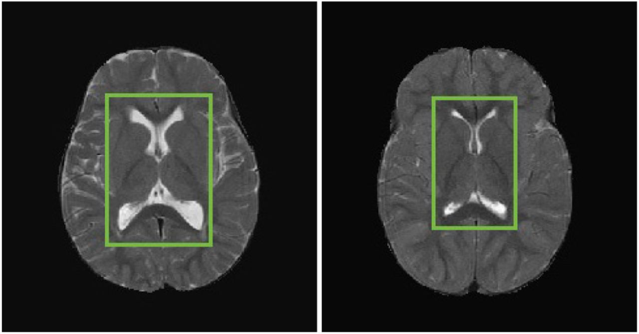
We hypothesized that severely increased brain volume would be associated with a smaller ventricular volume relative to the whole brain (Figure 2). As such, a measure of ventricular CSF requires the identification of ventricular and CSF voxels in the image.

Ventricular CSF volume and BV score. In these T2-weighted images, CSF is shown in the bright regions and ventricles are highlighted by green boxes. (Left) A subject with BV score = 2.5 indicating near-normal brain volume. (Right) A subject with BV score = 7 indicating highly increased brain volume.
To identify CSF regions, we leveraged a model of the observed intensities to partition voxels into classes. We used FSL FAST (Zhang, Brady and Smith, 2001), a popular approach that assumes that intensities and tissue classes can be modeled by a Gaussian Hidden Markov Random Field (GHMRF). Within the image for subject i, a voxel x can be classified as either gray matter, white matter, CSF, or none of these (extracerebral voxels). This assignment can be summarized by a tissue class segmentation function:

The collective tissue class assignments obtained by evaluating wi(x) at all voxels are denoted wi and must be estimated. In the GHMRF, both the observed voxel intensities viτ and the true tissue classes wi are considered to be random, and the goal is to find the class assignment wi maximizing their joint likelihood
 where the conditional distribution of viτ (x) | wi(x) is assumed to be Gaussian, and the tissue classes w are realizations of a Markov random field, and hence follow a Gibbs distribution.
However, the whole-brain CSF volume measurements have high variability among subjects, especially at the brain boundary; this is likely due to the brain segmentation performed in the previous step. Therefore, we limited the measure to ventricular CSF volume, which yielded a more stable estimate and demonstrated better identification of subjects with highly increased BV than either whole-brain CSF volume or ventricular volume alone. To segment the ventricles, we obtained adult ventricle atlases from the publicly available OASIS cross-sectional data set (Marcus et al., 2007). Using the same procedure of SyN registration and majority-voting label fusion as in the brain segmentation step, we obtained a ventricle mask for each subject, and calculated the ventricular CSF mask as the intersection of the CSF mask from FSL FAST and the OASIS ventricle mask.
For voxel x and subject i, we define the ventricular CSF mask function

The first image-based biomarker (Figure 3) is the brain parenchymal fraction (BPF) of the T2 scan, or the proportion of non-ventricular CSF voxels to total brain voxels:
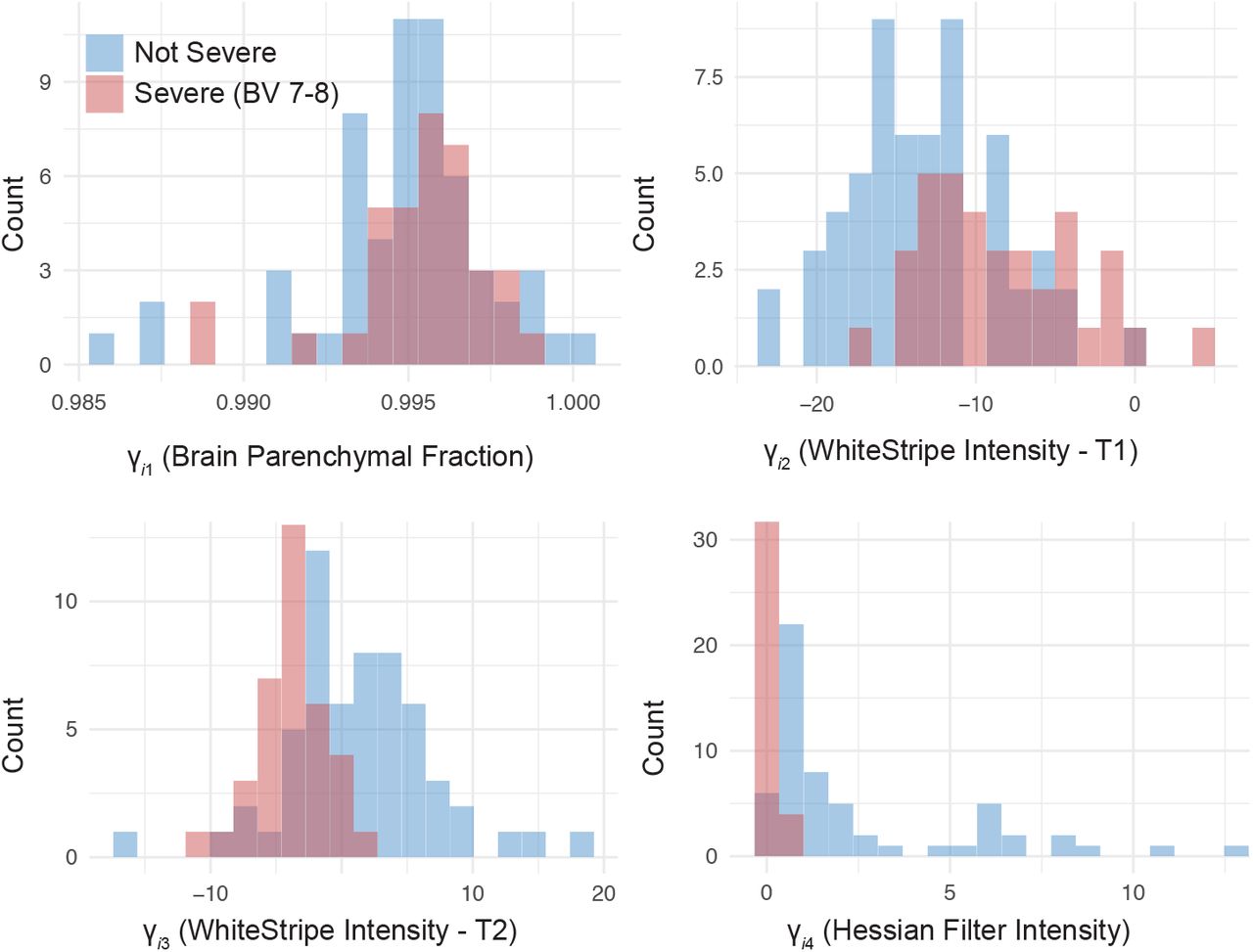
Distribution of derived biomarkers over all subjects in the sample and categorized by severe edema status.

Higher values of BPF represent a lower proportion of ventricular CSF volume and thus higher levels of brain swelling.
3.2.2. Grey-to-White Matter Differentiation
To translate the loss of gray and white matter delineation into a function of the observed image, it is necessary to normalize voxel intensities (within modalities) so that subjects can be compared. Therefore, for each subject, we applied a linear scaling of the image intensities based on normal-appearing white matter (NAWM) using the WhiteStripe technique (Shinohara et al. 2014).
For subject i and modality τ, the observed intensities viτ are assumed to follow a mixture distribution with K components. That is, the probability density f: ℝ→ ℝ is a function of intensity value v that decomposes as
 where the fik: ℝ →ℝ are subject-specific probability density functions and the weights yik sum to 1. It is assumed that there exists a transformation fik(v) → gk(v) so that the intensity distribution is not subject-specific:

The white stripe of NAWM is found by smoothing the empirical intensity histogram with a penalized spline (Ruppert, Wand and Carroll, 2003) and identifying the peak corresponding to white matter (in T1 scans this is the rightmost or highest-intensity peak; in T2 scans this is the overall mode). The interval around this peak, whose width may be adjusted by tuning parameters, is the white stripe. Every voxel intensity within the brain is then linearly scaled by the mode  and trimmed standard deviation
  of intensities within the white stripe:

Letting Bi equal the total number of brain voxels for subject i, we calculated the second and third biomarkers (Figure 3) using the T1 and T2 scans by taking the average normalized intensity after WhiteStripe within the brain voxels only (as determined by the brain segmentation mask in the previous section):

3.2.3. Sulcal Effacement
Finally, we considered that sulcal effacement, which is associated with BV scores of 6 to 8, might be extracted from the MRI by detecting gyri, or ridges, of the cerebral cortex (Figure 4). To do so, we used a filter on the Hessian matrix of each MRI image (Frangi et al., 1998).

Gyral features, such as sulci, are shown as bright in the T2-weighted MRI scan. (Top left) A subject with BV score = 2, which corresponds to decreased brain volume. (Top right) For a subject with BV score = 8 and severely increased brain volume, the sulci appear noticeably darker as they no longer contain CSF. (Bottom right) The Hessian filter is used to identify gyral features for a T2 image (bottom left) from a subject with BV score = 2.5.
In a 3-dimensional image, the Hessian matrix ℋiτ (x) at voxel x contains information about the local curvature around x for subject i and modality τ. Typically, ℋiτ (x) is calculated by convolving a neighborhood of x with derivatives of a Gaussian kernel. The three eigenvalues of ℋiτ (x) with smallest magnitudes  have a geometric interpretation: gyral or planar structures correspond to small values of
  and
and  and a high value of
  (Frangi et al., 1998). Tubular and spherical structures, on the other hand, are associated with different patterns in these eigenvalues, so the following dissimilarity measures are required to identify gyral features:

The vesselness image ℛiτ (x) is a function of these dissimilarity measures and other tuning parameters. By calculating its value at each voxel, we produced a probability-like map highlighting gyral features. We used the Hessian filter implemented in ITK-SNAP’s Convert3D tool (Yushkevich et al., 2006) on the T2 images, as they showed the best contrast between CSF and brain tissue. Due to limited field of view and the quality of brain segmentation around the top and bottom of the brain, the Hessian filter was only calculated in MRI slices taken from central portions of the cerebral hemispheres. The middle portion was defined by removing the top and bottom 3 slices (of the axial sequence) of each T2 image, as well as any voxels neighboring extracranial tissue (Figure 4).
We defined the final biomarker (Figure 3) as the median of the observed Hessian filter intensities in the T2 image limited to the brain voxels  defined by the erosion method above:
 The median was chosen as the distribution of the Hessian filter intensities within each image was highly right skewed; this resulted in a more conservative and robust characterization of the difference between severe and non-severe cases.
4. Prediction of Severe Brain Volume in Patients with CM
4.1 Model
To predict highly increased brain volume (a median BV score of 7 or higher), we defined the binary outcome variable for subject i and median BV score threshold k as the indicator variable  . The main outcome of interest in our study was
  . Together with the biomarkers introduced in the previous section, we formed the multivariate logistic regression model
 The estimated coefficients
  fit on the training set are shown in Table 2. Subjects with a BV score of 7-8 were associated with a lower median Hessian filter (p < 0.01), signifying fewer prominent sulci in the brain. This was the only coefficient found to be significantly different from zero, consistent with radiologists’ reports that sulcal effacement was the most important factor in determining a higher BV score. Both the intercept term and the coefficient of BPF had high standard errors, suggesting that there may have been near-complete data separation. For this reason, we did not interpret those coefficients.
Estimated coefficients in the prediction model (1) of severe brain edema.
4.2. Prediction Accuracy
In addition to model (1), we performed two sets of sensitivity analyses. The biomarkers γ·j for j ∈ {1, …, 4} were developed to identify images with BV ≥ 7; we considered an additional set of models with outcomes  and
and  , where the threshold for determining severely increased brain volume was relaxed. Because γi4, the measure of sulcal effacement, was both the most statistically and clinically important predictor of severe cases, we also considered models with γi4 alone (“Sulcal Only”) as opposed to the “Full Set” of covariates. In total, we examined 5 alternate models in addition to the main model, which are summarized in Table 3.
Prediction accuracy was assessed using area under the curve (AUC) and 95% confidence intervals for logistic regression models with binary outcomes  ,
,  , and
, and  (BV ≥7). We also considered models with either the full set of covariates in (1) (“Full Set”) or just the sulcal effacement biomarker (“Sulcal Only”). The primary model in (1) is shown in bold.
Prediction accuracy was assessed using area under the Receiver Operating Characteristic curve (AUC), which considers the sensitivity and specificity across different thresholds of the predicted outcome. For all models, the AUC was high, ranging from 0.81 to 0.96 in the training set, and 0.90 to 0.97 in the testing set. Models with outcome  received a lower AUC than those with outcome
  and
and  , although the 95% confidence intervals for all models intersect. This finding suggests—in corroboration with clinical observations—that patients with a BV score of 6 represent borderline cases and are therefore graded with the most uncertainty.
We compared models with γi4 as the sole covariate to the full model using a likelihood ratio test, and found that the reduced model performed similarly when the outcome was  (p > 0.3 in both training and test sets), moderately when the outcome was
  (p < 0.01 in the testing set only), and poorly when the outcome was
  (p < 0.01 in both training and test sets). In other words, the sulcal effacement biomarker was sufficient to classify cases scoring a 7 to 8, but all 3 biomarkers were needed to accurately classify cases with BV scores of 6 to 8. This suggests that the measures of ventricular CSF and gray-to-white matter differentiation, while less relevant for predicting cases scoring 7 or higher, may be useful in differentiating cases that were assigned a score of 5 versus 6.
In practical settings, a threshold on the predicted probability in model (1) is required to determine which individuals are predicted as severe or non-severe. To find an “ideal” threshold, we scanned a range of thresholds and chose that which maximized sensitivity and specificity in that order, with the restriction that specificity be greater than 0.90 (Table 4). Due to the discrete nature of the observations, the ideal threshold is not necessarily unique. For outcome  , the sensitivity was 0.78 and specificity was 0.96 using the full set of covariates; the sensitivity was 0.94 and specificity was 0.93 using just the sulcal effacement covariate. Together, these support the previous conclusion that sulcal effacement is the most important predictor for BV scores of 7 or higher. Furthermore, we identified a decision rule to distinguish severe and non-severe BV with low rates of false negatives and false positives. Indeed, a wide interval of acceptable thresholds, ranging from around 0.3 to 0.8, yielded acceptable values (> 0.75) of sensitivity, specificity, positive predictive value (PPV), and negative predictive value (NPV) (Table 4 and Figure 5). This suggests that, in clinical settings, the ultimate determination of severe or non-severe cases will have good accuracy that is robust to the choice of threshold.
Sensitivity and specificity of the prediction models. For each model, we considered a set of thresholds, where predicted probabilities greater than the threshold are interpreted as severe cases, and non-severe otherwise. Then, the final threshold was chosen such that the sensitivity and specificity were maximized, in that order, and with the restriction that specificity be greater than 90%. The primary model in (1) is shown in bold.
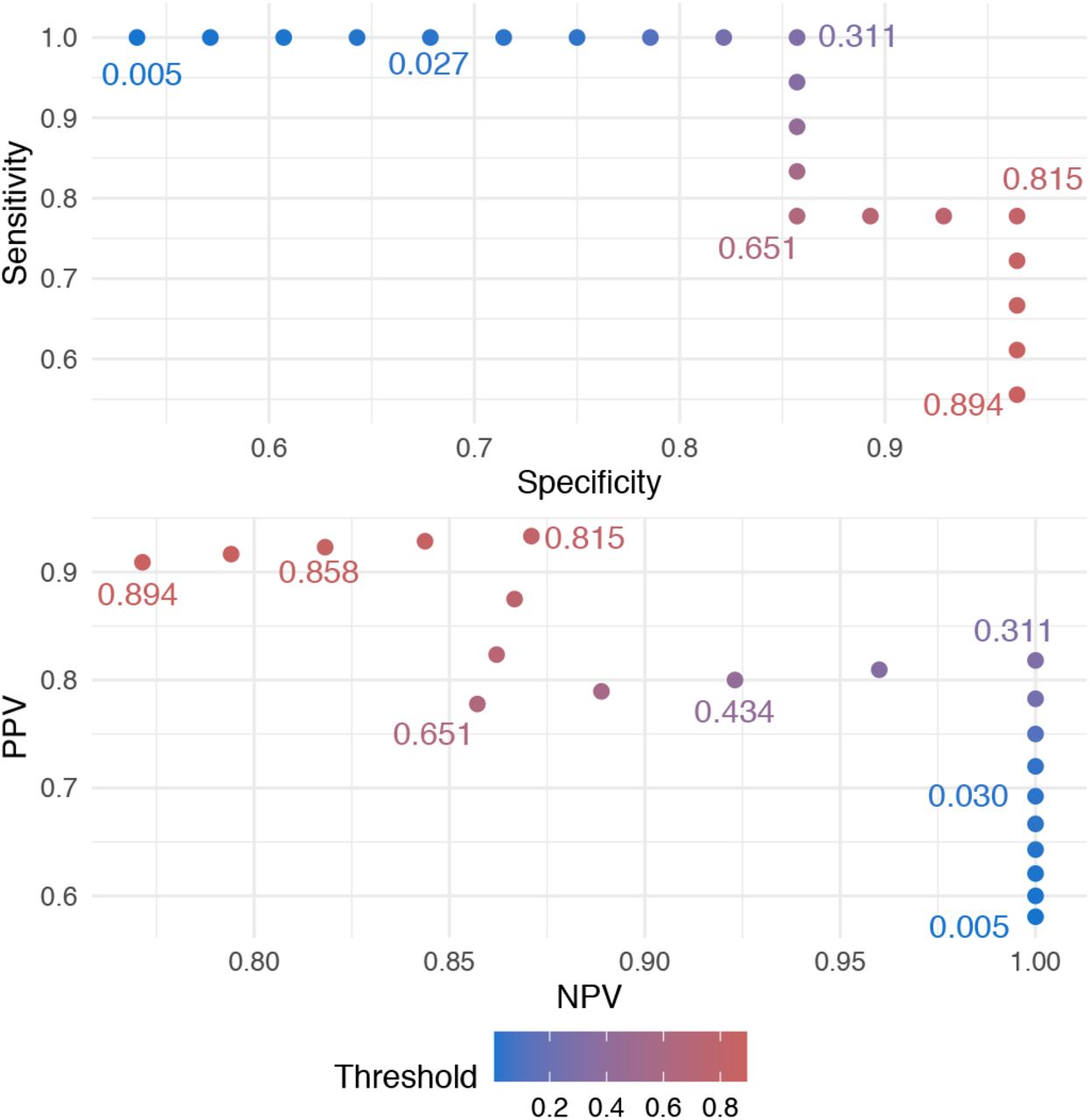
Given the primary model (1), the choice of threshold affects the sensitivity, specificity, positive predictive value (PPV), and negative predictive value (NPV) of the predicted outcome. We considered thresholds for which the sensitivity and specificity were higher than 50%. We found that a wide range of thresholds, ranging from around 0.3 to 0.8, yielded a favorable compromise between all four measures, while guaranteeing that each is higher than 75%. The data in this figure can be found in Supplementary Table S1.
4.3. Monte Carlo Validation
Although there were no known systematic clinical differences in the training and test set collection, there was a difference in the number of raters. To confirm that our results were not dependent on the initial split, we re-sampled the full dataset 100 times to form 100 training and test sets. In each re-sampling iteration, we fit the six aforementioned models using the training set and calculated the AUC (and 95% confidence interval) on the training and test set. Then, the average AUC (and 95% confidence interval endpoints) was calculated over the 100 iterations (Table 5).
Monte Carlo simulations demonstrate that our findings are not dependent on the initial split of training and test data. We re-sampled the data into training and test sets 100 times. Average AUC and average 95% confidence interval endpoints are shown for logistic regression models with binary outcomes  , and
, and  and either the full set of covariates in (1) (“Full Set”) or with the sulcal effacement biomarker (“Sulcal Only”). The primary model in (1) is shown in bold.
In the resampling schema, we observed the same pattern in prediction performance: over-all, classification accuracy was high for all models in both the training (mean AUC = 0.86-0.97) and test sets (mean AUC = 0.85-0.96). We again found that the Sulcal Only model performed as well as the full model for  and
and  , but notably worse than the full model for
  . Together, these results show that our derived biomarkers and model are able to accurately and robustly differentiate between subjects with highly increased brain volume (BV scores of 7 or 8) from those who do not. The measurement of sulcal effacement γi4 was again found to be the most important factor to identify cases with BV ≥7, with high average sensitivity, specificity, PPV, and NPV at selected thresholds of the predicted outcome (Table 6). Meanwhile, measures of ventricular CSF volume and gray and white matter differentiation γi1, γi2, γi3 provided more value in identifying “borderline” cases.
Sensitivity and specificity of the prediction models over 100 Monte Carlo simulations. As in Table 4, for each model and each re-sampling iteration, a range of threshold values were considered, along with the corresponding sensitivity and specificity of the predicted outcome. For each model and iteration, the maximum sensitivity and specificity were selected, in that order, with the restriction that specificity be greater than 90%. Then, these values were averaged across all 100 iterations in the training and test sets. The primary model in (1) is shown in bold.
5. Discussion
We have developed a method for the statistical image analysis of low resolution, noisy brain MRI, after determining that a popular method developed for images obtained on a high-field MRI scanner did not perform as well on the images in our sample. Our method involved creating and validating a multi-atlas, integrative framework to automate the radiological assessment of brain volume, a biomarker strongly associated with death in children with CM. Our logistic classification model is parsimonious, aligns with clinical observations, and has high predictive accuracy. The automated pipeline will be made available on GitHub as an R package that relies only on other open-source software. All high-resolution atlases for brain and ventricle segmentation are also publicly available resources, so other researchers can easily access the software and replicate our findings. An attractive feature of this program is that it requires only a subject’s T1- and T2-weighted MRI sequences as input in order to predict severe BV cases. One could further wrap the entire program in a Docker container in order to facilitate use and minimize conflicts due to computer settings. We hope that the implementation of these findings in low-resource environments can help to address both the shortage of radiologists for manual MRI interpretation, as well as the challenge of interpreting images from low-field MRI.
Our results provide insight into how radiologists score brain edema on MRI, generally supporting the stated importance of sulcal effacement over ventricular size and gray-to-white delineation. The superior performance of the sulcal effacement biomarker suggests that higher scores of brain edema were predominantly derived from this MRI feature, even as other features such as loss of gray-to-white matter delineation are also prescribed features for images assigned brain volume scores of 7 and 8. Future efforts to provide Hessian filter images or sulcal effacement scores might assist individual radiologists in producing more consistent gradings of brain volume. We intend to apply these methods to future analyses of brain MRI scans obtained with even lower field (< 0.1T) MRI scanners that are now being introduced in both high- and low-resource settings (Sheth et al., 2020) for clinical applications, including the evaluation of cerebral malaria.
A limitation of our approach is that logistic regression only accommodates binary outcomes (severe and non-severe brain volume scores); we did not predict the brain volume score itself. In exploratory analyses, models which predicted BV score directly had high misclassification error and mean squared error (results omitted), suggesting that more information or more sophisticated models may be needed to predict the ordinal score.
Future analyses could apply our pipeline to predict disease outcome: (Kampondeni et al., 2018) found that global CSF volume was the best predictor of prognosis in patients with CM. However, the accuracy of global CSF measurements in our current pipeline is limited by the quality of segmentation at the edge of the brain. Recent developments in deep learning methods for brain segmentation (Ronneberger, Fischer and Brox, 2015) could address this issue, although such procedures may require larger sample sizes with manual delineations of brain tissue than are currently available.
In summary, we introduced and validated a biologically and statistically principled method of biomarker development using images from low field strength MRIs, even in images with additional artifacts. We note that these strategies, which involve borrowing strength from publicly available high-resolution data whenever possible, and considering aggregate statistics that are more robust to extreme values, can be applied to any study of low-resolution brain images. The principles behind the tools introduced in this study are also broadly applicable to the design of new techniques that automate existing, clinically validated tasks.
Acknowledgements
The authors were supported by NIH Grants R01 MH112847, R01 NS112274, R01 AI034969, and R01 NS060910.
Footnotes
Sections 1 and 4 were updated to expand on clinical applications. Figure 5 and supplementary data were added.


