

Abstract
In order to analyse large complex stochastic dynamical models such as those studied in systems biology there is currently a great need for both analytical tools and also al-gorithms for accurate and fast simulation and estimation. We present a new stochastic approximation of biological oscillators that addresses these needs. Our method, called phase-corrected LNA (pcLNA) overcomes the main limitations of the standard Linear Noise Approximation (LNA) to remain uniformly accurate for long times, still main-taining the speed and analytically tractability of the LNA. As part of this, we develop analytical expressions for key probability distributions and associated quantities, such as the Fisher Information Matrix and Kullback-Leibler divergence and we introduce a new approach to system-global sensitivity analysis. We also present algorithms for statisti-cal inference and for long-term simulation of oscillating systems that are shown to be as accurate but much faster than leaping algorithms and algorithms for integration of diffusion equations. Stochastic versions of published models of the circadian clock and NF-κB system are used to illustrate our results.
- Abbreviations
- pcLNA,
- phase-corrected Linear Noise Approximation;
- KS,
- Kolmogorov-Smirnov;
- FIM,
- Fisher Information Matrix
1 Introduction
Dynamic cellular oscillating systems such as the cell cycle, circadian clock and other signaling and regulatory systems have complex structures, highly nonlinear dynamics and are subject to both intrinsic and extrinsic stochasticity. Moreover, current models of these systems have high-dimensional phase spaces and many parameters. Modelling and analysing them is therefore a challenge, particularly if one wants to both take account of stochasticity and develop an analytical approach enabling quantification of various aspects of the system in a more controlled way than is possible by simulation alone. The stochastic kinetics that arise due to random births, deaths and interactions of individual species give rise to Markov jump processes that, in principle, can be analyzed by means of master equations. However, these are rarely tractable and although an exact numerical simulation algorithm is available [1], for the large systems we are interested in, this is very slow.
It is therefore important to develop accurate approximation methods that enable a more analytical approach as well as offering faster simulation and better algorithms for data fit-ting and parameter estimation. A number of approximation methods aimed at accelerating simulation are currently available. This includes leaping algorithms [2, 3] and algorithms for integration of diffusion equation (or chemical Langevin equation (CLE)) [4] that provide faster simulation. However, these methods do not provide analytical tools for studying the dynamics of the system and they can also be extremely slow for data fitting and parameter estimation. One obvious candidate for overcoming these limitations is the Linear Noise Approximation (LNA). The LNA is based on a systematic approximation of the master equation by means of van Kampen’s Ω-expansion [5] which uses the system size Ω. Its large volume (Ω → ∞) validity has been shown in [6], in the sense that the distribution of the Markov jump process at a fixed finite time converges, as the volume Ω tends to ∞, to the LNA probability distribution. The latter distribution is analytically tractable allowing for fast estimation and simulation algorithms. However, the LNA has significant limitations, particularly, as we show below, in approximating long-term behaviour of oscillatory systems.
We show below that for the oscillatory systems that we study, the LNA approximation of the distribution Pt = P (Y (t)|Y (0)), of the state Y (t) of the system at some time t becomes inaccurate when the time t is greater than a few periods of the oscillation. However, if we rather consider a similar system which in the Ω → ∞ limit instead of a limit cycle has an equilibrium point that is linearly stable, then the LNA approximation of Pt remains accurate for a much longer time-scale. Linearly stable means that the eigenvalues of the system linearised at the equilibrium point have negative real parts. For example, in Fig. 3 of S3 we give an example where the LNA fails in a matter of a period or two for the oscillatory system, but for the corresponding equilibrium system it is very accurate for over a hundred times as long (and probably much longer). Similar behavior is also observed in other systems and using different measures in [7].
The observation that non-degenerate limit cycles have such linearised stability in the directions transversal to the limit cycle suggests the way forward for oscillatory systems. Our approach exploits the fact that, because of this transversal linearised stability, the distributionsPt for a general class of systems with a stable attracting limit cycle in the Ω → ∞ limit are, like the above fixed point systems, similarly well-behaved on long time-scales if one conditions Pt on appropriate transversal sections to the limit cycle.
We introduce a modified LNA, called the phase-corrected LNA, or pcLNA, that exploits the above observations to overcome the most important shortcomings of the LNA and develop methods for analysis, simulation and inference of oscillatory systems that are accurate for much larger times. We build on previous work of Boland et al. [8] which uses the 2-dimensional Brusselator system as an exemplar to investigate the failure of the LNA in approximating long-term behavior of oscillatory systems and presents a method for computing power spectra and comparing exact simulations with LNA predictions of the same phase rather than time. Other papers also employ a similar analysis to study the temporal variability of oscillatory systems in the tangental direction of the Ω → ∞ limit cycle [9] and/or the amplitude variability in the transversal direction of the limit cycle [10, 11, 12], using various low-dimensional oscillatory systems for illustration.
We extend these results in a number of ways including the following: (i) we develop a theory that treats the general case and provide analytical arguments that justify our approximations and enable computation of trajectory distributions, (ii) we show that the approach is practicable for larger nonlinear systems, (iii) we present a new powerful system-global sensitivity theory for such systems using measures such as the Fisher Information Matrix and the Kullback-Leibler divergence that are analytically computed, (iv) we present a simulation algorithm and show it is as accurate but faster than leaping and integration of diffusion equation algorithms, and (v) we derive the Kalman filter associated with the pcLNA in order to provide a practical way to accurately approximate the likelihood function thus facilitating estimation of system parameters θ and also for prediction. The approach in [8] uses transversal sections which are normal to the limit cycle. We follow this but in the supplementary information (Sect. 9 S1) we show that for most considerations one can use any transversal to the limit cycle.
To illustrate and validate our approach we apply it to a relatively large published stochastic model of the Drosophila circadian clock due to Gonze et al. [13] (see Sect. 1 S2). This model involves 10 state variables and 30 reactions. The oscillations are driven by the negative feedback exerted on the per and tim genes by the complex formed from PER and TIM proteins following phosphorylation. The per and tim mRNA is transported into the cytosol where it is degraded and translated into protein (P0 and T0). These proteins are multiply phosphorylated (PER: P0 → P1 → P2; TIM: T0 → T1 → T2) and these modifications can be reversed by a phosphatase. The fully phosphorylated form of the proteins is targeted for degradation and forms a complex, which is transported into the nucleus in a reversible manner where the nuclear form of the PER– TIM complex represses the transcription of per and tim genes. The large system limit is given by the differential equation system of 10 kinetic equations that are listed in the supplementary information (see Sect. 1 S2) along with the reaction scheme of the system.
The stochastic version of the Brusselator system and a stochastic version of a well-studied model of the NF-κB signalling system [14] are also used to illustrate our methods and the results can be found in S3. The supplementary information S1 contains technical derivations and S2, S3 further illustrative figures that we refer to in this paper.
2 Results
Stochastic models of cellular processes in signaling and regulatory systems are usually described in terms of reaction networks. A system of multiple different molecular subpopulations has state vector, Y (t) = (Y1(t),…, Yn(t))T where Yi(t), i = 1,…, n, denotes the number of molecules of each species at time t. These molecules undergo a number of possible reactions (e.g. transcription, translation, degradation) where the reaction of index j changes Y (t) to Y (t)+νj with the vectors νj ∈ ℝn called stoichiometric vectors. Each reaction occurs randomly at a rate wj (Y (t)) (often called the intensity of the reaction), which is a function of Y (t). Such systems can be exactly simulated using the Stochastic Simulation algorithm (SSA) [1].
The classical deterministic equations that describe the evolution of the concentration vector x(t) are derived by explicitly taking into account the volume Ω of the reaction system and assuming that the rates wj (Y (t)) depend upon Ω as wj (Y) = uj (Y /Ω, Ω). Here the dependence of uj on Ω is of canonical form in the sense of [5]. The limiting system as Ω → ∞ is given by a differential equation of the form
 where uj (x(t)) the limiting (Ω → ∞) deterministic rates (see Sect. 3 S1). Throughout we will be interested in the case where the solution x(t) of interest is a stable limit cycle γ of minimal period τ > 0 given by x = g(t), 0 ≤ t ≤ τ. We shall also always assume the generic situation for stable limit cycles in which all but one of the characteristic exponents of the limit cycle have negative real part [15] [16, Sect. 1.5].
Fig 1(A) displays a stochastic trajectory of the concentrations, X(t) = Y (t)/Ω, of two of the species of the circadian clock system obtained using exact SSA simulation over a period of time t ∈ [0, 8.5τ] (τ ≈ 26.98 hours). Here Ω = 300 is the volume of the system, imposing moderate to high levels of stochasticity. Results for system volumes Ω = 200, 500 and 1000 are also reported in Fig. 2 S2. Figure 1(B) shows realizations of the key probability distributions
 which describe the state of the system at some time t > t0. It is very rare that accurate analytical approximations for such probability distributions can be derived from the exact Markov-Jump process when t is large. Furthermore, as we can see, the SSA samples of P (X(t)|X(t0) = x0) spread along the curved periodic solution, x = g(t), of the limiting (Ω → ∞) deterministic system, implying that for large t this distribution is far from being normal and has a complex structure.

(A) A stochastic trajectory obtained by running the SSA over the time-interval t ∈ [0, 8.5τ] and (B) SSA samples (R = 3000) at times t = τ, 2τ,…, 8τ. Two (out of 10) of the species are displayed (per mRNA (x-axis) and nuclear PER-TIM complex (y-axis)). The volume size is Ω = 300. The black solid curve is the large volume, Ω → ∞, limit cycle solution.
However, we will show that there are important related distributions that can be well approximated even for large times t. For example, for each point x on the Ω → ∞ limit cycle γ, consider the (n − 1)-dimensional hyperplane N (x) normal to the limit cycle γ at x ∈ γ (i.e. orthogonal to the tangent vector F (x) at x) and the mapping GN defined by GN (X) = x ∈ γ if X ∈ N (x). If the system size is not too small, although there will be some reversals, the stochastic process GN (X(t)), t > 0, will move around γ in the direction of the deterministic flow given by (1) and, as t grows, GN (X(t)) will repeatedly pass by the value x every time the trajectory X(t) passes through the hyperplane N (X). In exact simulations, these intersection points,  , of X(t) with N (x), in round r = 1, 2,… are derived by interpolation between the last state before and the first state after the r-th intersection (see Sect. 2 S1). These points of intersection describe the stochasticity of the system around a particular phase x of the system. For example, the time at which the i-th variable is maximal in the deterministic system is given by the transversal submanifold Σ defined by
  so the intersection of the stochastic trajectory with this can be regarded as giving the statistics of the maxima of the stochastic trajectory (see Fig. 2(A)). Close to the limit cycle, Σ is well-approximated by its tangent space at the point of intersection with the limit cycle. Therefore, these distributions are useful for analysing various aspects of the system.

(A) Schematic representation of the intersections. (B) Quantile-Quantile (Q-Q) plots of the distribution of the fourth intersection,  , in transversal coordinates k = 2, 3,…, 10 (see Fig. 3 S2 for r = 1, 2,…, 8). (C) KS distances between the empirical distribution of the intersections
  for the first r = 1, 2,…, 7 rounds of the stochastic trajectory and the distribution
  in the final round (r = 8), k = 2, 3,…, 10.
Our first observation is that the empirical transversal distributions
 obtained by exact simulation are approximately normal (Fig 2(B)). Moreover, as r increases
  and
and  are hardly distinguishable and appear to converge to a fixed, approximately normal transversal distribution as r increases (Fig. 2(C)). Similar results hold if we use a different family of transversal sections to γ as explained in Sect. 10 S1.
2.1 The Linear Noise Approximation (LNA)
This naturally raises the question of whether asymptotic approximation methods such as the LNA, which provide multivariate normally distributed approximation of the stochastic system, can be used to accurately approximate these transversal distributions.
The LNA as formulated by [6] is derived directly from the underlying Markov jump process and is valid for any time interval of finite fixed length. It is based on the ansatz
 where x(t) is a solution of the limiting (Ω → ∞) deterministic system (1). In our case we always take x(t) to be the periodic solution g(t). A key aspect of this ansatz is that ξ(t) satisfies a linear stochastic differential equation (SDE) that is independent of Ω, with drift and diffusion matrices that are functions of the deterministic solution g(t). Details are given in Sect. 4 S1.
Given an initial time t0 and an initial condition for ξ(t0) the LNA determines the distributions, of ξ(t), t > t0, and hence  that we respectively denote by PLNA(ξ(t)|t0, ξ(t0)) and PLNA(X(t)|t0, ξ(t0)). If ξ(t0) is only known up to a multivariate normal (MVN) distribution P0 then we denote these distributions, respectively, by PLNA(ξ(t)|t0, ξ0 ∼ P0) and PLNA(X(t)|t0, ξ0 ∼ P0) (see Fig 4). Details of how to calculate these are given in Sect. 4 S1.
Each of the above distributions is MVN enabling analytical approaches for example in analysing the stochastic sensitivities of the system. If we fix t > t0 then as Ω → ∞ the true distribution of ξ converges to the distribution PLNA(ξ(t)|t0, ξ(t0)) (see e.g. [5]). However, one most certainly cannot reverse the limits i.e. for a fixed Ω one cannot expect the approximation to hold for large time t → ∞. This is certainly the case when the LNA is used with oscillators and we aim to overcome this by developing methods that remain accurate for much larger times than the LNA.
We first consider the distribution P (X(t)|X(0) = x0) and compare this for SSA simulated samples and the LNA at a sequence of times t = τ, 2τ,…, 8τ and for an arbitrary (fixed) initial state x0 ∈ γ. As we can see in Fig. 3, the LNA fits the SSA simulations relatively well in the short run (t = τ), but as time progresses the Kolmogorov-Smirnov (KS) distance between the two distributions for each state variable for the LNA and SSA increases substantially beyond the threshold level (see Fig. 3(B)). The LNA predictions spread along the tangental direction and therefore fail to accurately reflect the SSA samples that have spread along the curved limit cycle.

(a) Samples obtained from the SSA simulation algorithm (red crosses) and 0.01, 0.05, 0.40 contours of the LNA probability density (black ellipsoids) at fixed times, t = τ, 2τ,…, 8τ (τ: minimal period), for the circadian clock system. The limit cycle ODE solution is also displayed (black solid line). (b) KS distance between the empirical distribution of SSA samples and LNA distribution of each species (different colors, see legend) at the fixed times. The threshold level is also displayed (black solid line). The system size is Ω = 300.

 as r increases. The yellow distribution represents the limit as r → ∞. Although, for free oscillators, the latter distribution diverges the corresponding conditional distributions converge.
On the other hand, as we saw earlier, the transversal distributions  are approximately normal. We next derive an approximation of
  under the LNA and show that it accurately approximates
  in the Drosophila circadian clock, Brusselator and NF-κB systems. Importantly, this pcLNA approximation is MVN and therefore it enables the analytical study of various aspects of the system.
2.2 Calculating transversal distributions
We firstly consider how to approximate the transversal distribution
 where x1 = g(t1), t1 > t0, and P0 is a MVN distribution supported on the normal N (g(t0)). This is the distribution of intersection points of stochastic trajectories with the section N (g(t1)). To approximate
  we take PLNA(X(t1)|t0, ξ(t0) ∼ P0) and calculate the conditional distribution
  given by conditioning on X(t1) ∈ N (g(t1)). Since PLNA(X(t1) |t0, ξ(t0) ∼ P0) is MVN this conditioning is relatively simple and done using the Schur complement (Sect. 5-6 S1). It gives a MVN distribution supported on N (x1). Now suppose that we have calculated
  . Then,
  is
is  conditioned on X(t1 + τ) ∈ N (x1) where τ is the period of γ.
Note that  is also given by conditioning PLNA(X((r − 1)τ + t1) |t0, ξ(t0) ∼ P0) on X((r − 1)τ + t1) ∈ N (g(t1)) because the LNA is transitive i.e. for all t1, t2 > 0,

In S1 we show that, although PLNA(X((r − 1)τ + t1) |x0, ξ0 ∼ P0) diverges as  converges exponentially fast to a distribution
  (Sect. 7 S1, cf. Fig. 4). The distribution
  is a fixed point in the sense that
  conditioned on
  . Using this fact enables us to calculate
  directly because, as we show in the SI, its mean and covariance matrix satisfy a simple fixed point equation that is easily solved numerically (Sect. 8 S1).
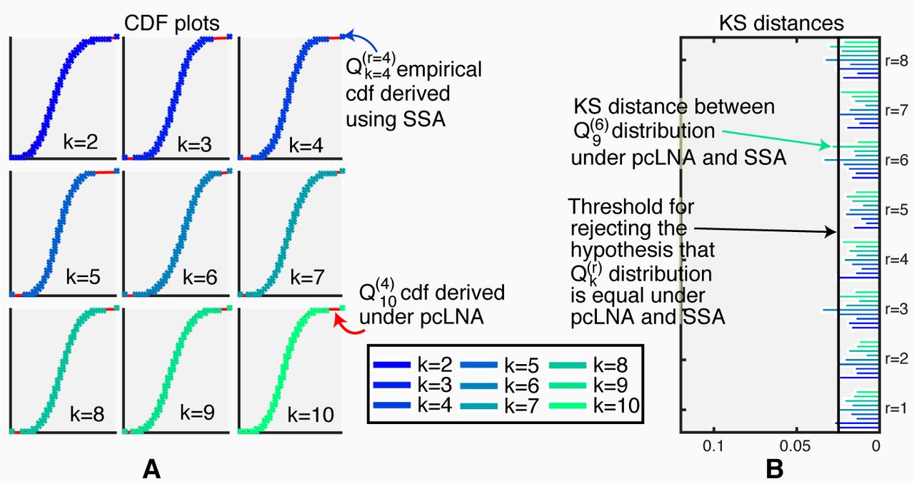
The question remains as to how well these distributions capture the exact simulation transversal distribution  . This is addressed in Fig. 5 where it is shown that the fit is excellent even for Ω as low as 300. The fit is even better for higher system sizes (Fig. 5 S2). In S3 we also show similar low Ω results for the Brusselator (Fig. 2 S3) and the NF-κB system (Fig. 5 S3). Thus we note that although the LNA cannot be used directly to accurately compute P (X(t)|X(0)) for a fixed Ω and increasing t, using it to compute the transversal distributions provides accurate estimates of
  for much larger times t1+ rτ. Moreover, in Sect. 7 S1 we also explain why the convergence of the distribution on normal hyperplanes implies convergence on other transversal sections to γ. However, this result only applies to free-running oscillators and does not apply to forced oscillators as is explained there.

(A) CDF plots of the transversal distributions  under the pcLNA (red line) and the SSA (empirical cdf, crosses) for transversal coordinates k = 2, 3,…, 10 and round r = 4 (see Fig. 4 S2 for r = 1, 2,…, 8). (B) KS distances between the
  distributions under pcLNA and SSA, r = 1, 2,…, 8, k = 2, 3,…, 10.
The covariance structure of  is very interesting and accurately represents the co-variance structure of the distribution
  obtained from exact simulations. The variances in the direction of the principle axes rapidly decrease. On the other hand, the variances of the individual state variables at these same points on γ are much more uniform in their sizes (Fig 1).
Next, we describe the pcLNA joint distribution of multiple intersections to possibly different transversal sections on the limit cycle. This is MVN and has parameters in a relatively simple form.
2.2.1 Joint distribution of multiple transversals
Consider q phase states of the limit cycle xi = g(ti), i = 1, …, q, on γ where 0 ≤ t1 < t2 <… < tq < τ. If X(t) is a stochastic trajectory, we consider how it meets the transversal sections at the xi as t increases. As mentioned above, if the system size is not too small, although there will be some reversals, GN (X(t)) will move around γ in the direction of the deterministic flow given by (1) and so we can talk of the times when GN (X(t)) first takes the phase xi during the r-th revolution of GN (X(t)) around γ. Suppose it first meets Sx in  for i = 1, …, q. If i < q then we let
  denote the first point in
  that X meets after it leaves
  . If i = q then the next transversal it meets is
  and the intersection point is
  In this way we derive a sequence of points
  .
.
We shall be interested in the distribution

Remarkably, in our approximation, this distribution is MVN with a covariance matrix whose inverse has a simple tridiagonal form in terms of the drift and diffusion matrices coming from the LNA (Sect. 8 S1).
The fact that the above transversal distributions are MVN allows us to analytically compute the Fisher Information matrix and associated quantities that can be used to perform a stochastic sensitivity analysis of oscillatory systems.

The stochastic trajectory X(t) (blue line), initiated from x0, intersects each of the transversal sections Sx1, Sx2 and Sx3 (dashed lines) of the limit cycle (red solid line) three times, following a path  .
.
2.3 Fisher Information
Fisher Information quantifies the information that an observable random variable carries about an unknown parameter θ. If P (X, θ) is a probability distribution depending on parameters θ, the Fisher Information Matrix (FIM) I = IP has entries
 where l = log P, and θi and θj are the i-th and j-th components of the parameter θ. If P is MVN with mean and covariance µ = µ(θ) and Σ = Σ(θ) then

The FIM measures the sensitivity of P to a change in parameters in the sense that
 where DKL is the Kullback-Leibler divergence. The significance of the FIM for sensitivity and experimental design follows from its role in (5) as an approximation to the Hessian of log-likelihood function at a maximum. Assuming non-degeneracy, if θ∗ is a parameter value of maximum likelihood there is a s × s orthogonal matrix V such that, in the new parameters θ′ = V · (θ − θ∗),
 for θ near θ∗. From these facts it follows that the
  are the eigenvalues of the FIM and that the matrix V diagonalises it. If we assume that the σi are ordered so that
  then it follows that near the maximum the likelihood is most sensitive when
  is varied and least sensitive when
  is. Moreover, σi is a measure of this sensitivity.
The theory of optimal experimental design is based on the idea of trying to make the σi decrease as slowly as possible so that the likelihood is as peaked as possible around the maximum, thus maximising the information content of the experimental sampling methods. Various criteria for experimental design have been proposed including D-optimality that maximises the determinant of the FIM and A-optimality that minimise the trace of the inverse of the FIM [6]. Diagonal elements of the inverse of FIM constitute a lower-bound for variance of any unbiased estimator of elements of θ (Cramer-Rao inequality). However, for the systems we consider here the σi typically decrease very fast and there are many of them. Thus, in general, criteria based on a single number are more likely to be of less use than consideration of the set of σi as a whole.
Calculation of the FIM for stochastic systems using the LNA has been carried out in [17] but only for small systems and short times where the LNA is accurate. It is notable that the pcLNA enables one to do this for large systems and large times. As an example, we analyse the stochastic behavior of the circadian clock based on the limit distribution  when
when
 where x0 = g(t0) and x1 = g(t1) are chosen so that t0 is the time of the peak of per mRNA MP and t1 the peak of the nuclear complex of PER and TIM proteins CN. We compute the Fisher Information of the latter distribution using the closed form expression (Sect. 7.3 S1) for this distribution. As we can see in Fig. 7(A) the eigenvalues of the Fisher Information matrix decay exponentially, with a sharp decline followed by a slower decrease. This reveals that the influential directions in the parameter space of the system are much less than its total dimension. Furthermore, a few parameters appear to be most influential. The eigenvectors associated with the two largest eigenvalues of Fisher Information matrix (see Fig. 7(B)) have large entries only for the parameters kdn (PER-TIM complex nuclear degradation), kd (per mRNA linear degradation), k2 (PER-TIM complex transportation to cytosol), vst (tim mRNA transcription), kip (per mRNA Hill coefficient) and kit (tim mRNA Hill coefficient).
The exponential decrease of the eigenvalues is typical of tightly coupled deterministic systems [18, 19, 20, 21, 22, 23, 24], but has to our knowledge not been demonstrated before for stochastic systems. It has important consequences. For example, it tells us that only a few parameters can be estimated efficiently from time-series data unless the system is perturbed in some way to get complementary data and that there will be identifiability problems that can be analysed using the FIM. It also can be used to design experiments that will give data so that the FIM of the combined models (old and new experimental data) will alleviate the decline of the eigenvalues.
2.4 Sensitivity analysis for stochastic systems
The fact that we can calculate the Fisher Information allows a new approach to sensitivity analysis for stochastic systems. As above we consider a family of probability distributions P (X, θ) which we assume are MVN with mean µ(θ) and covariance matrix Σ(θ) depending on the parameters θ. We show that there is a natural matrix of sensitivities Sij associated with such a system. These are system-global in that they look at how all components of the systems change with parameters. They also have an intimate relationship with Fisher information.
As is well-known in Information Geometry the set of multivariate normal distributions MVNn on ℝn can be given the structure of a Riemannian manifold in which the Riemannian metric is given by the line element

Points in MVNn are denoted by Θ = (µ, Σ) where µ is the mean and Σ the covariance matrix. The corresponding inner product in the tangent space at Θ0 = (µ, Σ) is given by
 where δΘj = (δµj, δΣj), j = 1, 2.
In calculating the FIM we have to determine the partial derivatives ∂µ/∂θi and ∂Σ/∂θi. The derivative M of the mapping θ → (µ(θ), Σ(θ)) at a parameter value θ0 is given by
 where the derivatives are calculated at θ0.
We can regard M as a linear mapping between the parameter space ℝs and MVNn with the inner product given in equation (7). We can then prove (Sect. 10 S1) that we can find s orthonormal vectors Vi spanning the parameter space ℝs, s orthonormal vectors Ui in the space MVNn and numbers σ1 ≥ · · · ≥ σs such that


(A) The logarithm of the eigenvalues of the Fisher Information Matrix (FIM). (B) The entries/weights of the eigenvectors corresponding to the 2 largest eigenvalues of FIM (C) The largest principal control coefficients Sij. Small values are reduced to 0.
Note that the orthonormality of the Ui is with respect to the inner product 〈⋅,⋅〉Θ0. The eigenvalues of the FIM F are the squares of the σi because with respect to the standard inner product on θ-space and 〈⋅,⋅〉Θ0 on MVN the adjoint M∗ satisfies M* M = F (Sect. 10 S1).
If we let  denote the decomposition of Ui into µ and Σ components, then the following key property follows from (8): if δθ is any change of parameters, the change in µ and Σ is given by
 where Sij = σiVji.
One can define other sensitivities in a similar way but using a different orthogonal basis of MVNn, but the above Sij satisfy an important optimality condition explained in Sect. 10 S1 which asserts that the basis Ui and the corresponding sensitivities Sij are optimal for capturing as much sensitivity as possible in the low order principal components Ui. In view of this we call the Sij the principal control coefficients. Note that the role of the Sij as sensitivities is seen from the following relation which follows from (9),

These sensitivities are relatively easy to calculate using the information in Sect. 10 S1. In Fig. 7(C) we show the Sij for the transversal distribution of the drosophila circadian clock at the times of the peak of per mRNA and the peak of the nuclear complex of PER and TIM proteins. As we can see, because Sij = σiVji the coefficients rapidly decrease with the singular values σi, while a few parameters, similar to those with large eigenvector entries, have high coefficients.
2.5 pcLNA Simulation Algorithm
Given the ability to accurately approximate the transversal distributions and the results in [8] we realised it should be possible to use this to construct a rapid simulation algorithm. The approach is to use resetting of g(t) to GN (X(t)) to cope with the growth in the variance of g(t) − GN (X(t)) and keep the LNA fluctuation in the transversal direction. The fact that g(t) − GN (X(t)) is expected to be approximately normal (see Sect. 11 S1) enables us to do this in a well-defined way.
The pcLNA simulation algorithm is described next. Its main step is illustrated in Fig. 8.
Choose a time-step size δτ > 0.
Input initial condition κ(t0) and X(t0) = g(t0) + Ω−1/2κ(t0).
For iteration i = 1, 2,…
sample ξ(ti−1 + δτ) from MVN(Ciκ(ti−1), Vi);
compute Xi = g(ti−1 + δτ) + Ω−1/2ξ(ti−1 + δτ);
set ti to be such that GN (Xi) = g(ti) and κ(ti) = Ω1/2(Xi − g(ti)).
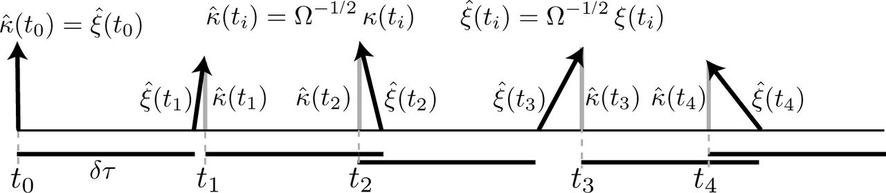
The solid horizontal bars below the horizontal axis are all of length δτ, the basic timestep of the algorithm. The black arrows show  and the grey arrows
  . Having calculated
  one uses κ(ti) as the initial state and updates it using the LNA and a time-step δt to obtain ξ at ti + δt. Then ξ is replaced by κ so that g(ti + δt) + Ω−1/2ξ = g(t) + Ω−1/2κ where κ is normal to the limit cycle. Lastly, ti+1 = t and
  .
.
In the for loop Ci = C(ti−1, ti−1 + δτ) and Vi = V (ti−1, ti−1 + δτ) are the drift and diffusion matrices in the linear SDE describing the evolution of the noise process ξ(t) under the LNA (see Sect. 4 S1).
If one wants to record simulated trajectories at a finer time-scale than δτ then one can run the algorithm with δτ replaced by δτ /M for some integer M > 1 and only carry out the phase correction in step 3(c) every M th step and at all the other steps just proceeding as in the standard LNA (ignoring step 3(c)). This gives the same distribution as if the intermediate points had not been calculated because of the transitive nature of the LNA i.e. PLNA(X(s + t)|X(0)) = PLNA(X(t)|X(s) ∼ PLNA(X(s)|X(0))). In the simulation results described below, the time-step δτ = 6 hours and M = 3 so that there are τ /6 ≈ 4.5 corrections in every round of the limit cycle. The effect of less frequent correction is studied in Sect. 4.1 S2. The pcLNA algorithm is fast because (i) it can make relatively large steps from one transversal distribution to another maintaining accurate temporal correlation, and (ii) because, although it has to integrate the variational equation of the system (Sect. 4 S1), there is an efficient method to compute and store a subset of the drift C(s, t) and diffusion V (s, t) matrices for the system and the given parameters once and for all so that all required variational solutions can be computed extremely quickly from this subset. This subset is computed up-front. A Matlab routine to do this is contained with the package PeTSSy which is freely available (Sect. 12 S1). Thus, the only extra computational cost compared to the standard LNA is due to the calculation of GN (X) which can be practically performed through an optimization procedure (e.g. the Newton-Raphson algorithm).
2.5.1 Comparisons to other simulation algorithms
We compared the pcLNA simulation algorithm in terms of both CPU time and precision of the approximation with some of the most important alternatives, the tau-leap method and the integration of the chemical Langevin equation (CLE) method. Exact simulations produced by the SSA are also used as a reference for the comparison.
For the tau-leap simulation we use the algorithm described in [3], which is a refinement of the original tau-leap method first proposed in [2]. In [3] the authors suggest an optimal method to compute the largest possible time step such that the leap condition is still approximately satisfied. The leap condition ensures that the state change in any time step is small enough so that no rate function will experience a macroscopically significant change in its value. The error of this approximation is controlled by a parameter ∈. For integrating the CLE described in [4], we use the classical Euler method (see [25]) with a fixed time step δt.
For both the tau-leap and the CLE approximation we explored different values of their parameters ε and δt, respectively, to attain a good balance of precision and CPU time. Here we present the results for the largest values of both ε and δt, hence smallest CPU time, which attain similar performance with the pcLNA algorithm in terms of precision. If little improvement could be achieved in terms of precision by lowering either ∈ or δt, the larger values are preferred.
The algorithms are implemented for a fixed time-interval (8.5 times the period of the limit cycle of the system) and the comparison is made at 8 fixed time points using the KS distances between the empirical distribution of each algorithm and the empirical distribution derived using the SSA simulations. Note that for all approximation algorithms, the probability of generating negative populations is non-zero and there are a number of methods for dealing with this. Our simple approach is described in Sect. 13 S1.
Figure 9 displays the median CPU times for a single trajectory simulation in t ∈ [0, 8.5τ], under the competing approaches for different system sizes, Ω = 300, 1000, 3000, along with a comparison in terms of precision for Ω = 300 (see Fig. 7, 8 S2 for Ω = 1000, 3000, respectively). A sample of size R = 2000 is produced for each algorithm. We see that the precision of all approximation methods is fairly similar, with their empirical distributions almost indistinguishable to exact simulations. In terms of CPU times, we see that the SSA is much slower than the other algorithms particularly for large system sizes. The tau-leap offers some improvement to the CPU times but this is relatively small compared to the CLE approximation and especially the pcLNA algorithm. One reason for this relatively small improvement for the tau-leap algorithm is the stiffness of the considered system, a property that is however very common in biological systems and it is known to slow down the tau-leap method by requiring small values of the ∈ parameter to ensure that the leap condition is satisfied and hence the approximation is fairly precise. Note that for similar reasons, a small δt was necessary to achieve good precision with the CLE approximation.
The pcLNA algorithm is about 24 times faster than the CLE approximation and much faster than the tau-leap and the SSA. In our simulations, it took 0.4sec to derive this long-time trajectory, which means that in about 7 minutes one can generate more than 1000 trajectories of this large system over a long-time compared to about 2.7 hours with CLE approximation and much longer times for the other methods. Therefore, the pcLNA offers a substantial improvement in CPU times compared to standard approaches in simulating oscillatory systems without compromising the precision of the simulation substantially. Perhaps more importantly, it is based on a framework which one can also use to analyse oscillatory systems and perform statistical inference. For the latter the following Kalman filter is particularly relevant.

Panels (A), (B) and (C) contain the samples produced by respectively the pcLNA, tau-leap (∈ = 0.002) and CLE (δt = 0.002) algorithms and the exact simulation (SSA) at time-points, t = 1τ, 2τ,…, 8τ, for Ω = 300, along with the KS distances between the empirical distributions of each approximation and the SSA for each system variable (colored bars). Panel (D) provides the median CPU times for a single trajectory run in the time-interval [0, 8.5τ] under the different simulation algorithms along with the ratio of the median CPU time under SSA and each approximation algorithm.
2.6 Calculating likelihoods via a pcLNA Kalman Filter
Although there is no elegant formula for
 similar to
  above, we can efficiently calculate it. To do this we derive a Kalman Filter for the pcLNA that is a modification of the Kalman Filter associated with the LNA [26]. This can be used to compute the likelihood function
  of the system parameters θ with respect to observations
  recorded at N times t0, t1, …, tN that are noisy linear functions of the species concentrations. This is slightly more general than just calculating
  because we allow for a measurement equation. The Kalman filter can also be used for forward prediction.
We assume the measurement equation,
 relating the observations
  to the state variables, X(t). Here B is a transformation matrix (often simply removing unobserved species or introducing unknown scalings) and ϵ = (ϵ1,…, ϵn) ∼ M V N (0, Σ ϵ) the observational error. The pcLNA likelihood can be decomposed as

Let m(t) and S(t) be the mean and covariance matrix of the stochastic process  under the LNA. Then µ(t) = g(t) + Ω−1/2m(t) and Σ(t) = Ω−1S(t) are the mean and covariance matrix of X(t) and
  <the mean and covariance of
  . Denote
  the prediction error at time t.
The pcLNA Kalman Filter algorithm uses the following recursive algorithm for computing the terms in  . Note that (µ∗, Σ∗) denote posterior estimates of (µ, Σ) conditional on the observed measurement at the current time.
Input
 , B and Σϵ.
Compute
from M V N .For iteration i = 1, 2,…
Derive
;Compute
;Derive
;Compute
from .


In the for loop  , and
, and
 where the matrix ∈2(t) = [e2(t) … en(t)] has columns orthonormal vectors which are also orthogonal to the unit tangent vector e1(t) = F (x(t))/‖F (x(t)) ‖ and

The measurement equation (11) is used to derive the predictive probabilities  and
and  in steps 2 and 3(d), respectively. The posterior distribution
  in step 3(a) is derived by Bayes rule, while the posterior distribution of the corrected noise process
  in step 3(b) is derived by restricting the posterior distribution of the noise process on the transversal section
  normal to e1(t′) using the Schur complement as described earlier. The cartesian coordinate system is used here. If this correction is omitted, step 3(b) of the above algorithm is replaced by the standard LNA step,
  where
where  .The LNA Ansantz (Eq. 3) and transition (Eq. 4.3 S1) are used to derive the prior distribution
  in step 3(c).
3 Discussion
We present a comprehensive treatment of stochastic modelling for large stochastic oscillatory systems. Practical algorithms for fast long-term simulation and likelihood-based statistical inference are provided along with the essential tools for a more analytical study of such systems. There is considerable scope for future work in various directions. We expect that these results can be extended to a broader class of systems including those that are chaotic in the Ω → ∞ limit. Our approach should provide the opportunity to develop new methodology for parameter estimation, likelihood-based inference and experimental design in such systems. Finally, there is currently much interest in information transfer and decision-making in signaling systems and our methods provide new tools with which to tackle problems in this area. If system biologists are to reliably use complex stochastic models to provide robust understanding it is crucial that there are analytical tools to enable a rigorous assessment of the quality and selection of these models and their fit to current biological knowledge and data. Our aim in this paper is to contribute to that but the results should be of much broader interest.
Supporting Information
S1 Appendix
Technical Details
In this note we give further details about the mathematical underpinnings of the pcLNA methods discussed in the main paper.
S2 Appendix
Drosophila Circadian Clock system
In this note we give details about the drosophila circadian clock and use this system to illustrate further the accuracy of distributions and simulations discussed in the main paper.
S3 Appendix
Brusselator and NF-κB systems
In this note we give details about the deterministic and stochastic models of the Brusselator and NF-κB systems and use them to illustrate further the results described in the main paper.
Acknowledgments
This research was funded by the BBSRC Grant BB/K003097/1 (Systems Biology Analysis of Biological Timers and Inflammation). DAR was also supported by funding from the European Union Seventh Framework Programme (FP7/2007-2013) under grant agreement n ° 305564.
References


