

Abstract
Background This paper re-analyzes the gene set data from [1] and [2] which purportedly showed 3 opposing effects of hedonic and eudaimonic happiness on the expression levels of a set of genes that 4 have been correlated with social adversity.
Methods Four non-parametric methods were used to test the two null hypotheses addressed in the original studies ( and
and  ) as well as the null hypothesis of no difference in effect between hedonic and eudaimonic happiness (
 ).
).
Results Standardized effects (mean partial regression coeffcients) of Hedonia and Eudaimonia on gene expression levels are very small in both the 2013 and 2015 data, as well as the combined data. The p-values from all four tests are similar in magnitude and fail to reject any of the null models.
Discussion The results unambiguously fail to support opposing effects, or any detectable effect, of hedonic and eudaimonic happiness on the pattern of gene expression. The apparently replicated pattern of gene expression is simply “correlated noise” due to the geometry of multiple regression given the strongly correlated measures of hedonic and eudaimonic happiness.
Background
In a highly visible gene set analysis, Fredrickson et al. 2013 [1] claimed that a measure of eudaimonic happiness was associated with a decreased “conserved transcriptional response to adversity” (CTRA) while a measure of hedonic happiness was associated with increased CTRA. This transcriptional response includes the up-regulation of pro-inflammatory signals and the down-regulation of antiviral and antibody synthesis signals. Brown et al. [3] criticized multiple components of the methodology and interpretation of Fredrickson et al. 2013 [1], including importantly here, the one-sample t-tests of the set of regression coefficients of the CTRA genes on hedonic and eudaimonic scores. Fredrickson et al. 2015 [2] followed up the criticism of [3] with a replicate study but using a marginal model with a specified correlated errors matrix, to estimate the associations between CTRA gene expression and happiness scores. In this follow-up study, Fredrickson et al. 2015 [2] showed that the pattern of mean CTRA gene expression replicated that of Fredrickson et al. 2013 [1] but that only eudaimonic happiness had a statistically significant effect on CTRA gene expression.
Here, I present the results of a re-analysis of the Fredrickson et al. 2013 [1] and Fredrickson et al. 2015 [2] data. Not being a social psychologist, I limit my analysis to addressing the question “what is the evidence for effects of hedonic and eudaimonic happiness scores on CTRA gene expression” and give here only the necessary background to understand my analysis. The CTRA gene set includes 19 pro-inflammatory, 31 anti-viral, and 3 antibody-stimulating genes. The Fredrickson et al. 2013 [1] data included all 53 genes but the Fredrickson et al. 2015 [2] data is missing IL-6 from the pro-inflammatory subset.
Fredrickson et al. 2013 [1] used 53 univariate multiple regressions to estimate the effects (the regression coefficient) of each happiness (hedonic and eudaimonic) score on log2(normalized gene expression) for each gene. The regression model included both happiness scores, seven covariates to adjust for demographic and general health confounding (sex, age, ethnicity, BMI, a measure of alcohol consumption, a measure of smoking, and a measure of recent illness), and eight covariates to adjust for immune status confounding (expression level of T-lymphocyte markers). Hedonic and eudaimonic scores were transformed to z-scores prior to the analysis. The 53 multiple regressions (one for each gene) yielded 53 coefficients for hedonic score and 53 coefficients for eudaimonic score. The coefficients of the 31 anti-viral and 3 antibody genes were multiplied by -1 to make the direction of the effect consistent with the CTRA response. Fredrickson et al. 2013 [1] used a simple one-sample t-test of the 53 coefficients to test for a mean effect of hedonic or eudaimonic score on CTRA expression. A mean coefficient greater than zero reflects a positive CTRA response (increased pro-inflammatory and decreased anti-viral and antibody-stimulating genes).
The fundamental problem with the Fredrickson et al. 2013 [1] t-test is that the coefficients are not independent of each other because of the correlated expression levels among genes. As a consequence of the correlated error, a one-sample t-test of the coefficients violates the test’s assumption of independent error. One way to think about the consequence of this violation is to consider a null model of no effect of happiness score on any of the 53 genes. The mean absolute correlation in the 53 × 53 correlation matrix of Fredrickson et al. 2013 [1] gene expression levels is 0.25. The maximum is 0.92. Because of the high correlations among the expression levels, a set of 53 coefficients computed with the hypothetical null data will tend to have either more positive or more negative signs than expected. Consequently, the error of the mean coefficient (the standard error) is much larger than if the coefficients were independent. And, as a consequence, there will be an inflated Type-I error in a one-sample t-test of the mean. Brown et. al. [3] discovered this inflated Type-I error in their exploration of the Fredrickson et al. 2013 [1] data.
In response to criticism from Brown et. al. [3], Fredrickson et al. 2015 [2] used a generalized least squares (GLS) model with a heterogenous compound symmetry error matrix, effectively treating each of the 52 gene expression levels as repeated measures of a common effect [2]. I am not aware of any criticism or re-analysis of Fredrickson et al. 2015 [2]. While a GLS estimate of marginal effects is consistent even if the error correlation is misspecified, the variance of the estimates will be biased. Compound symmetry assumes equal correlation (conditional on the set of predictors) among all expression levels. This is not likely to approximate the true error structure for a set of expression levels for different genes, as these expression levels will share different sets of underlying regulatory factors. A second and perhaps more fundamental problem with the Fredrickson et al. 2015 [2] analysis is the small sample size (n = 122 or n = 198 in the combined data) relative to the number of regression coefficients (69) and variance parameters (53) that must be estimated. This small sample per parameter ratio is likely to result in overfit models, which, in turn, will result in unstable and inflated coefficients [4]. Typically, when only the fixed effects are of interest (as here), the fixed effects and their errors are estimated using Generalized Estimating Equations instead of GLS to avoid issues resulting from estimating the correlated error matrix [5, 6]. Finally, and most importantly, the GLS model gains power by assuming that the estimated regression coefficient is a common effect for all genes (and each univariate estimate is merely an estimate of this common effect), an assumption that is more appropriate for longitudinal or repeated measures than for multiple outcomes such as gene expression levels.
The general question addressed by Fredrickson et al. 2013 [1] and Fredrickson et al. 2015 [2], that is, is there a mean response different from zero for a set of multiple outcomes, has a long and rich history in applied statistics [7], including in association studies of gene sets[8, 9]. Bull [10] is an especially clear exposition of the different null hypotheses that one might test. Wu et al. [11] clearly outline some of these hypotheses in the context of gene set associations.
Here, I reanalyze the Fredrickson et al. 2013 [1] data (hereafter, FRED13), the Fredrickson et al. 2015 [2] data (FRED15), and the combined data (FRED13+15) using both bootstrap resampling to obtain standard errors of effects that account for the correlated expression levels and permutation tests to test the null hypotheses of zero mean effects for Hedonia and Eudaimonia. The re-analysis includes a permutation version of the O’Brien OLS test [7] and a randomization procedure implemented for gene set analysis [11]. The results from all analyses for each datasets are consistent in that they all fail to provide evidence against the nulls. Additionally, I show that the high correlation (.79 and .73 in the two datasets) between the two focal predictors (Hedonia and Eudaimonia) results in coefficients with negatively correlated errors that may be misinterpreted as a “replicable” pattern instead of correlated noise reflecting the geometry of multiple regression.
Methods
Data were downloaded as .txt Series Matrix Files from http://www.ncbi.nlm.nih.gov/geo/ using accession numbers GSE45330 and GSE55762. The CTRA (response) expression data were log2 transformed. The T-lymphocyte expression data that formed part of the set of covariates were log2 transformed in the downloaded data. The downloaded hedonic and eudaimonic scores in FRED13 had means and variances close but not equal to that expected of z-scores, which suggests that the public data slightly differs from that analyzed by Fredrickson et al. 2013 [1]. Three rows of FRED13 had missing covariate data (two rows were completely missing) and were excluded; the number of rows (cases) in the cleaned matrix was 76. The downloaded hedonic and eudaimonic scores in FRED15 were the raw values and were transformed to z-scores. There was no missing data in FRED15 and the number of cases was 122.
Prior to all analyses, the expression levels of the 31 anti-viral and 3 antibody genes were multiplied by -1 to make the direction of the effect consistent with the CTRA response [1, 2].
Null hypothesis tests
The overall effect of Hedonia or Eudaimonia on expression levels of the CTRA gene set is simply the averaged effect over all genes,  . Two of the focal null hypotheses that are tested here, which were also the focus of Fredrickson et al. 2013 [1] and Fredrickson et al. 2015 [2] are
  and
and  . Fredrickson et al. 2013 [1] and Fredrickson et al. 2015 [2] also discussed the differential effect of Hedonia and Eudaimonia on CTRA gene expression but inferred this from differences in p-values. Here I explicitly test the null hypothesis of no difference in effect between the two types of happiness using the null hypothesis
  . I refer to these three null hypotheses as
  , and
, and  .
.
All three hypotheses are directional, that is, the mean effect differs from zero. This differs from the general multivariate test that at least one of the coefficients differs from zero, but the mean response may be zero. While the hypotheses are directional, the tests are two-tailed, that is, the mean response may be up or down regulation of the CTRA gene set.
Inferential tests
The effects of Hedonia and Eudaimonia on the mean of the m gene expression levels are estimated with the multivariate linear model
 where Y is the n × m matrix of gene expression levels for the n subjects, X is the model matrix of dummy variables and covariates, E is the matrix of residual error, and B is the p × m matrix of partial regression coefficients. The coefficients of the jth column of B are precisely equal to univariate multiple regression of the jth gene on X (and why the model is sometimes called a multivariate multiple regression). In R, estimating the m effects of Hedonia and Eudaimonia is much faster using this multivariate model than looping through m univariate multiple regressions. I refer to the mean of the m coefficients as the OLS estimates.
Four tests were used to test the null hypotheses. In all four tests, the happiness scores for Hedonia and Eudaimonia and the m expression levels were mean-centered and variance-standardized. Consequently, the reported OLS estimates are the mean standard partial regression coefficients (averaged over the m genes).
Procedural bootstrap t-Test
Fredrickson et al. 2013 [1] used a bootstrap resampling method to compute a p-value. In their bootstrap, the 53 partial regression coefficients were re-sampled with replacement 200 times. Each iteration, a mean regression coefficient was computed. The standard deviation of the 200 means was used as the estimate of the standard error to compute a t-statistic and associated p-value. Resampling the regression coefficients fails to address the lack of independence among the coefficients. To estimate the sampling error that accounts for correlated error among the regression coefficients, the entire estimation procedure needs to be included within the bootstrap by resampling the data and re-estimating the coefficients. In each iteration of this procedural bootstrap, entire rows of the data were re-sampled with replacement, the m coefficients were estimated by equation 1, and the re-sampled mean coefficients ( and
and  ) were saved each iteration. 1999 bootstrap iterations were run. The t-statistic for each hypothesis is the observed mean coefficient (
 , or
, or  for the difference in means) divided by its standard error, which was estimated as the standard deviation of the 2000 saved mean coefficients.
Permutation t-test
As an alternative to the bootstrap t-test, I used permutation to generate null distributions of t-statistics for each null hypothesis and then computed p-values from these null distributions. To comply with the assumption of exchangeable error, I followed Anderson and Robinson [12] and used the permutation method of Freedman and Lane[13]. For this procedure, the predictor variables were divided into main effects Z (hedonic and eudaimonic scores) and covariates X (the demographic and immune variables). Using the non-permuted data, the observed residuals (EY) and predicted values  of Y|X were estimated using equation 1. For each of the permuted iterations, rows of EY were permuted and added to the non-permuted
  to generate a permuted response
  , where π indicates a permuted value. Prior to fitting the permuted data, Hedonia and Eudaimonia and the m expression levels were re-centered and variance-standardized. The m coefficients for both Hedonia and Eudaimonia were then computed from the model
  and
and  was computed from the m coefficients for each of the three hypotheses. Additionally, a t-statistic was computed for each hypothesis each iteration using
 where sβ is the standard deviation of the m coefficients. 2000 iterations were run, including an iteration of non-permuted data. The two-sided p-value of each hypothesis was computed as the fraction of |tperm| ≥ the observed |tperm|.
Permutation O’Brien’s OLS t-Test
Neither the bootstrap t-test nor permutation test explicitly accounts for the correlation among the regression coefficients (although both implicitly account for this in the resampled distributions). To explicitly account for this correlation, I used a modification of O’Brien’s OLS test [7]. After standardizing the covariates and all gene expression levels to unit variance, O’Brien’s test statistic is
 where j is a m vector of 1s, t contains the t-statistic associated with each of the m partial regression coefficients, and R is the correlation matrix of the m coefficients. More simply, the numerator is the sum of the t-statistics for each gene and the denominator is the sum of all of the elements of R. R was estimated using a bootstrap resampling procedure. The null distribution of tObrien was constructed using the observed value and 1999 permutations of the data. The permutation procedure was exactly that for the permutation t-test above except that each iteration of the permutation, the permuted data was resampled and refit (using Equation 1) 1000 times in order to estimate R as the correlation matrix of the 1000 × m set of coefficients. The inner and outer loops make this a computationally intensive test.
Rotation Gene Set Test (ROAST)
The final test of  is the rotation-test described in Wu et al. [11] and implemented in the function roast from the limma package [14]. The test statistic, zrot, is a mean z-score computed from the set of m moderated t-statistics computed for each gene. Using a hierarchical model, the moderated t-statistic uses information on the error of all genes in the set to estimate the gene specific standard error. A p-value for the test statistic is evaluated in a very similar manner to that described above in “Permutation test” but with some key differences. First, in the rotation-test, the observed residuals (EY) are from Y|X where X includes not only the covariates but also the non-focal happiness score (for example, Eudaimonia is included in X for the test of Hedonia). Second, instead of permutation, the n-vector of residuals is rotated by a random vector r, which is constant for all genes within each iteration but variable among iterations. And third, the rotated residuals
  are used to directly compute the new t-statistics and z-scores without fitting the new model
  (where π indicates rotated residuals). The observed and rotated z-scores from 1999 rotations were used to generate the null distribution. The p-value for the “UpOrDown” test was used as this is the test of the two-tailed directional hypothesis.
Permutation Generalized Least-Squares
If we assume the separate coefficients for each of the m genes is an estimate of a common effect β, then the tests described above lose power due to effectively discarding the m within subject estimates of β. A fixed-effects marginal model potentially gains power by using all nm responses but avoids pseudoreplication [15] (or inflated Type I error) by weighting the standard error of the estimate by the within subject error covariance matrix. To implement this model, the data matrix is stacked into long format by combining the m expression levels into a single variable expression and the variable Gene is created to identify the gene associated with a specific expression value. The fixed-effects marginal model is
 where yi is the vector of m responses for subject i, Xi is the model matrix for subject i, which includes the main effect Gene to identify the jth element of yi, and β is the vector of coefficients, including the common effects of each covariate on the response. In this model,
  , where Σ is the within subject error covariance matrix.
While the “common effect” assumption is highly questionable for gene expression data, it is useful to explore this model in order to learn about the results from Fredrickson et al. [2]. Following Fredrickson et al. 2015 [2], I used GLS with a heterogenous compound symmetry error matrix to estimate the common effects (βHedonia and βEudaimonia. Exploration of the behavior of the GLS suggested very unstable coefficients and, consequently, I used a bootstrap procedure to show this sensitivity to sampling and a permutation test to estimate p-values. Each iteration of either the bootstrap or permutation, the data was resampled (permuted) in wide format, rescaled, and reshaped to long format. For both bootstrap and permutation, the coefficients were estimated using the gls function from the nmle package [16]. In both, the first iteration used the observed (not resampled or permuted) data. The bootstrap was limited only to the combined FRED13+15 data because of lack of convergence issues with the smaller datasets. 500 iterations of the bootstrap procedure were run (including the iteration with the observed sample). For the permutation test, the standard partial regression coefficients and associated t-statistics for Hedonia and Eudaimonia were saved each iteration and used to generate a null distribution of expected values (using the t-statistic) given no effect of either on expression level. Due to the time required to fit the GLS, only 300 permutations were run but this was sufficient to get an approximate p-value. To estimate the sensitivity of this p-value to only 300 permutations, 95% confidence intervals were computed for the p-value using 2000 bootstrap resampled sets of the 300 permutation t-statistics.
Type I error in the GLS method
I used Monte Carlo simulation to explore the inflation of type I errors due to overfitting in the GLS fit using the parametric estimate of the standard error. In each run of the simulation, a random nxp matrix X of independent variables (n samples of p covariates) and a random n × m matrix Y of response variables (n samples of m responses) were generated using the function rmvnorm from the mvtnorm package [17]. All simulated independent variables were modeled as continuous variables sampled from 𝒩(0, SX), where SX is the covariance matrix of the 17 regressor variable from FRED15. The 52 response variables were modeled as continuous variables sampled from 𝒩(0, SY), where SY is the covariance matrix of the 52 gene expression levels from FRED15. The expected effect of any of the X on any of the Y is zero.
To reduce the time required for the simulation, subsets of m =10, 20, or 30 of the 52 response variables were sampled randomly. p is the number of covariates (17) from FRED15. The sample size was determined as n = 2(m +p). Because the number of regressors is m + p (again, the data are in long format), the ratio of samples to regressor was 2 for all runs. This ratio is in-between that for FRED15 and the combined data (1.8 and 2.9, respectively). 200 iterations of each subset were run. The p-values associated with the t-test of the coefficients for the two X variables simulating Hedonia and Eudaimonia (that is, with an expected correlation equal to that in FRED15) were saved each iteration.
All analyses were performed using R [18]. All data cleaning and analysis scripts are available at the public GitHub repository https://github.com/middleprofessor/happiness.
Results
Replication of previous analyses
Fredrickson et al. 2013 [1] do not report either the partial regression coefficients of each gene expression level on hedonic and eudaimonic score or the mean coefficient for each score. The back-transformed mean effects ( × 100, where
  is the mean of the m coefficients) for all three datasets are given in Table 1. My values approximate the values inferred from Fig. 3 of Fredrickson et al. 2015 [2] with the exception of that for Hedonia from FRED13, which is noticeably smaller than that figured in Fredrickson et al. 2015 [2]. This likely reflects small differences between the public data and thta analyzed in Fredrickson et al. 2013 [1] [see also 3]. From the p-values based on a t-statistic that assumes independence of the regression coefficients (Table 1), one might reasonably reject each null hypothesis for each dataset.
Back-transformed mean effect sizes ( × 100) and naive p-values from the 2013, 2015, and combined data
The variance-standardized effects and p-values for hedonic and eudaimonic scores estimated from the GLS for each dataset are given in Table 2. My coefficients for FRED15 are the same as those reported in Fredrickson et al. 2015 [2] to the 3rd decimal place. My coefficients for the combined data are similar to my coefficients for the FRED15 data, while Fredrickson et al. 2015 [2] report a substantially smaller negative effect for Eudaimonia for the the combined data. Again, this is likely due to small differences between the public FRED13 data and the data actually analyzed in [1].
GLS estimates of the variance-standardized coefficients for the 2013, 2015, and combined data. The bootstrap standard error and permutation p-values are also given
Importantly here, the coefficients for the FRED13 data have the opposite pattern of that for FRED15 and combined data, that is, with the 2013 data, the effect of Hedonia is large and has a very small p-value (0.002) while the effect for Eudaimonia is small and not statistically significant (p = 0.44).
New results
Standardized mean effects ( ) are very small and positive for Hedonia and very small and negative for Eudaimonia for all three datasets (Table 3). The bootstrap SE for each mean indicates that a 95% confidence interval is too large to have any confidence in the direction of either of the effects for any dataset. The p-values computed using the the procedural bootstrap, the permutation t-test, the permutation O’Brien’s t-test, and the rotation z-test are very consistent and all fail to reject the null. The OLS estimates of the difference (∆) between hedonic and eudaimonic effects are small and positive. The bootstrap SE for all ∆ are too large to have any confidence in the direction of the difference and the p-values from each of the four tests fail to reject the null for any of the data sets.
OLS estimates of mean Hedonia and Eudaimonia effects on CTRA gene expression. The esti-mates are the mean variance-standardized partial regression coefficients from the multivariate regression over the m responses (genes). The SE was estimated using a bootstrap. The p-values are from the bootstrap, permutation t, permutation Obrien’s t, and rotation z tests.
OLS estimates of the difference in effect  for the 2013, 2015, and combined data. The SE was estimated using a bootstrap. The p-values are from the bootstrap, permutation t, permutation Obrien’s t, and rotation z tests
GLS stability
The GLS coefficients were described above (Table 2). The bootstrap standard errors for the FRED13+15 data for the GLS fit are over twice the parametric estimates (Table 2), which shows that the coefficients are very sensitive to sampling. Again, bootstrap errors were not computed for FRED13 or FRED15 because of too many issues with convergence of the smaller datasets. Despite the large coefficient for Eudaimonia for FRED13+15, the standard errors are too large to have any confidence in the direction of the effect. The p-values from the permutation test fail to reject any of the nulls.
The large bootstrap relative to parametric standard errors for the GLS coefficients suggest an inflated Type I error rate with the parametric p-values. Type I error for the GLS parametric p-values for simulated data modeled on FRED15 is given for different levels of α in Table 5. The results show highly inflated Type I error which increases with smaller α.
Type I error and Inflation factor  for the GLS test of Fredrickson et al. 2015 [2]. The Error is the average of the error computed for the simulated coefficients for Hedonia and Eudaimonia
Discussion
The re-analysis of the gene expression data in subjects scored for hedonic and eudaimonic happiness unambiguously fails to support either the original conclusion of an opposite relationship of hedonic and eudaimonic happiness on the CTRA (conserved transcriptional response to social adversity) gene set [1] or the more recent conclusion limiting the relationship to eudaimonic well-being [2]. The consistency among the four different tests for each hypothesis and dataset is notable. The p-values from the permutation
O’Brien’s t-test and rotation Z test are especially close despite the differences in the implementation of the randomization. That said, the rotation test is very fast relative to the permutation O’Brien test, which required nested re-sampling.
The apparent replication of the sign of the effects between FRED13 and FRED15 [2] is true for the OLS estimates but strikingly false for the GLS estimates, although this failure of the GLS test to replicate was not noted by Fredrickson et al. [2] because they used the OLS estimate and not the GLS estimate to show the replicated pattern of expression. Regardless, any replication in the sign of the mean effect should not be surprising given only two replicates of two coefficients. More importantly, as I show below, the apparent replication is expected given the high correlation between hedonic and eudaimonic scores.
Beyond the fact that a GLS model with 69 predictors and 53 variance estimates was fit with a mere 122 (FRED15) or 198 (FRED13+15) subjects, several features of the results suggest inflated coefficient estimates resulting from overfitting the model to noise. First, at least one of the GLS coefficients in each of the datasets is very large relative to what we’d expect from a gene set association given observational data and the stated hypotheses. Second, the GLS coefficients are very different from the OLS coefficients (Tables 2 and 3). Third, the opposite pattern of effects estimated in FRED13 and FRED15 suggests that either something very different biologically is going on between the subjects in FRED13 and FRED15 or the coefficients are very unstable due to a combination of overfitting and multicollinearity. Fredrickson et al. 2015 [2] did not report re-analyzed results for FRED13 using the GLS model so do not discuss either interpretation. Fourth, the plot of residuals against the predicted values shows a strong, negative relationship (not shown). And finally, the Type I error rate of the simulated data modeled on FRED15 is highly inflated (Table 5). Especially striking about the Type I error rates is the relatively high frequency of very small p-values (p ≤ 0.001).
The conclusions of Fredrickson et. al. 2015 [2], then, are based on p-values from tests contaminated by highly inflated Type I errors due to overfitting combined with moderate multicollinearity and a high correlation between the two focal predictors. The consequences of the highly correlated focal predictors has not been discussed in detail. Fredrickson et al. 2015 [2] emphasized the replicated pattern of a positive mean coefficient (described in the introduction) for Hedonia and a negative mean coefficient for Eudaimonia, where a positive coefficient implies up-regulation of the genes associated with social adversity. This pattern and apparent replication is almost certainly a function of the multicollinearity among the predictors in combination with the high positive correlation between hedonic and eudaimonic scores. It is well known that the partial regression coefficients of two highly correlated predictors are negatively correlated (one will tend to be positive and the other negative), which is the case with these data. For example, using FRED13, and disregarding all predictors but hedonic and eudaimonic scores, the partial regression coefficient of any gene expression level on Hedonia (X1) and eudaimonoia (X2) are
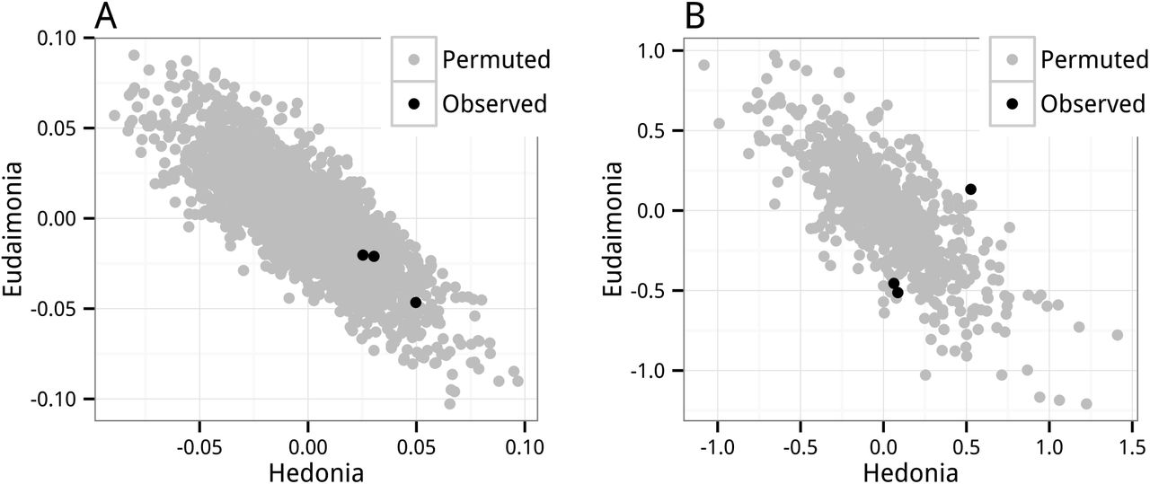
 where the 2.66 and -2.1 are the diagonal and off-diagonal elements of the inverse of the correlation matrix with .79 in the off-diagonal (the correlation between hedonic and eudaimonic scores in FRED13). Because of the high correlation, both β1 and β2 include a large contribution from the covariance of the other X and Y but the sign of this contribution is negative. Consequently, if the expected xTy is zero for both predictors, the β coefficients will be negatively correlated. Random noise creates negatively correlated error. This negative correlation is easily seen in the scatterplot of βhedonia vs. βeudaimonia for the gene IL1A (the choice ofgene doesn’t matter) from the permutation t-test (Figure 1A). The negative correlation is also seen using the coefficients from GLS model, which estimates a single coefficient for the complete set of genes (Figure 1B). In both of these analyses, the expected effects (partial regression coefficients) are zero (because of the permutation) yet the estimates are negatively correlated. Note that this correlated error arises from the correlation between hedonic and eudaimonic scores (Equation 5) and is not the same as the correlated error that arises from the correlation among the gene expression levels. Unambiguously, then, the data from Fredrickson et al. 2013 [1] and Fredrickson et al. 2015 [2] do not show a replicated pattern of differentially expressed genes associated with social adversity between hedonic and eudaimonic people. Instead, this apparently replicable pattern of differential expression is simply correlated noise arising from the geometry of multiple regression.

Coefficients from permuted runs are in grey. Observed coefficients for all three datasets are in black. The expected effects for the permuted runs is zero. A. Partial regression coefficients of IL1A from the permutation t-test. B. Partial regression coefficients (accounting for the expression of all genes simultaneously) from the permutation GLS model.
References


