

Abstract
A model which treats the denatured and the native conformers as being confined to harmonic Gibbs energy wells has been used to analyse the non-Arrhenius behaviour of spontaneously-folding fixed two-state systems. The results demonstrate that when pressure and solvent are constant: (i) a two-state system is physically defined only for a finite temperature range; (ii) irrespective of the primary sequence, the 3-dimensional structure of the native conformer, the residual structure in the denatured state, and the magnitude of the folding and unfolding rate constants, the equilibrium stability of a two-state system is a maximum when its denatured conformers bury the least amount of solvent accessible surface area (SASA) to reach the activated state; (iii) the Gibbs barriers to folding and unfolding are not always due to the incomplete compensation of the activation enthalpies and entropies; (iv) the difference in heat capacity between the reaction-states is due to both the size of the solvent-shell and the non-covalent interactions; (v) the position of the transition state ensemble along the reaction coordinate (RC) depends on the choice of the RC; and (vi) the atomic structure of the transiently populated reaction-states cannot be inferred from perturbation-induced changes in their energetics.
Introduction
It was shown elsewhere, henceforth referred to as Papers I and II, that the equilibrium and kinetic behaviour of spontaneously-folding fixed two-state systems can be analysed by a treatment that is analogous to that given by Marcus for electron transfer.1-3 In this framework termed the parabolic approximation, the Gibbs energy functions of the denatured state ensemble (DSE) and the native state ensemble (NSE) are represented by parabolas whose curvature is given by their temperature-invariant force constants, α and ω, respectively. The temperature-invariant mean length of the reaction coordinate (RC) is given by mD-N and is identical to the separation between the vertices of the DSE and the NSE-parabolas along the abscissa. Similarly, the position of the transition state ensemble (TSE) relative to the DSE and the NSE are given by mTS-D(T) and mTS-N(T), respectively, and are identical to the separation between the curve-crossing and the vertices of the DSE and the NSE-parabolas, respectively. The Gibbs energy of unfolding at equilibrium, ΔGD-N(T), is identical to the separation between the vertices of the DSE and the NSE-parabolas along the ordinate. Similarly, the Gibbs activation energy for folding (ΔGTS-D(T)) and unfolding (ΔGTS-N(T)) are identical to the separation between the curve-crossing and the vertices of the DSE and the NSE-parabolas along the ordinate, respectively.
The purpose of this article is to use the framework described in Papers I and II to analyse the non-Arrhenius behaviour of the 37-residue FBP28 WW domain, at an unprecedented range and resolution.4
Equations
The expressions for the position of the TSE relative to the vertices of the DSE and the NSE Gibbs parabolas are given by

 where the discriminant φ = λω + ΔGD-N(T) (ω − α), and λ = α(mD-N)2 is the Marcus reorganization energy for two-state protein folding. The expressions for the activation energies for folding and unfolding are given by

 where the parameters βT(fold)(T) (= mTS-D(T)/mD-N) and βT(unfold)(T) (= mTS-N(T)/mD-N) are according to Tanford’s framework.5 The expressions for the rate constants for folding (kf(T)) and unfolding (ku(T)), and ΔGD-N(T) are given by


 where, k0 is the temperature-invariant prefactor with units identical to those of the rate constants (s−1), R is the gas constant, T is the absolute temperature. If the temperature-dependence of ΔGD-N(T) and the values of α, ω, and mD-N are known for any two-state system at constant pressure and solvent conditions (see Methods), the temperature-dependence of the curve-crossing relative to the ground states may be readily ascertained. The temperature-dependence of curve-crossing is central to this analysis since all other parameters can be readily derived by manipulating the same using standard kinetic and thermodynamic relationships.
The activation entropies for folding (ΔSTS-D(T)) and unfolding (ΔSTS-N(T)) are given by the first derivatives of ΔGTS-D(T) and ΔGTS-N(T) functions with respect to temperature

 where TS is the temperature at which the entropy of unfolding at equilibrium is zero (ΔSD-N(T) = 0) and ΔCpD-N is the temperature-invariant difference in heat capacity between the DSE and the NSE.6 The activation enthalpies for folding (ΔHTS-D(T)) and unfolding (ΔHTS-N(T)) may be readily obtained by recasting the Gibbs equation: ΔH(T) = ΔG(T) + TΔS(T), or from the temperature-dependence of kf(T) and ku(T) to give


The difference in heat capacity between the DSE and the TSE (i.e., for the partial unfolding reaction [TS] ⇌ D) is given by

Similarly, the difference in heat capacity between the TSE and the NSE (for the partial unfolding reaction N ⇌ [TS]) is given by

The reader may refer to Papers I and II for the derivations.
Results and Discussion
As mentioned earlier and discussed in sufficient detail in Papers I and II, the analysis we are going to perform has an explicit requirement for a minimal experimental dataset which are: (i) an experimental chevron obtained at constant temperature, pressure and solvent conditions (except for the denaturant); (ii) an equilibrium thermal denaturation curve obtained under constant pressure, and in solvent conditions identical to those in which the chevron was acquired but without the denaturant, using either calorimetry or spectroscopy; and (iii) the calorimetrically determined ΔCpD-N value (i.e., the slope of the linear regression of a plot of model-independent ΔHD-N(Tm) vs Tm, where ΔHD-N(Tm) is the enthalpy of unfolding at the midpoint of thermal denaturation, Tm; see Fig. 4 in Privalov, 1989).7 Fitting the chevron to a modified chevron-equation using non-linear regression yields the values of mD-N, the force constants α and ω, and the prefactor k0 (k0 is assumed to be temperature-invariant; see Methods in Paper I). Fitting a spectroscopic sigmoidal equilibrium thermal denaturation curve using standard two-state approximation (van’t Hoff analysis using temperature-invariant ΔCpD-N) yields van’t Hoff ΔHD-N(Tm) and Tm and enables the temperature-dependence of ΔHD-N(T), ΔSD-N(T) and ΔGD-N(T) functions to be ascertained across a wide temperature regime (Eqs. (A1)-(A3), Figure 1 and Figure 1−figure supplement 1).6 Once the values of mD-N, the force constants, the prefactor, and the temperature dependence of ΔGD-N(T) are known, the rest of the analysis is fairly straightforward. The values of all the reference temperatures that appear in this article are given in Table 1.

(A) Temperature-dependence of ΔGN-D(T), ΔHN-D(T), and TΔSN-D(T). The green pointers identify Tc and Tm. The slopes of the red and black curves are given by ∂ΔGN-D(T)/∂T=-ΔSN-D(T) and ∂ΔHN-D(T)/∂T=ΔCpN-D, respectively. (B) An appropriately scaled version of plot on the left. The reference temperatures are as described in the parent figure.

(A) Temperature-dependence of ΔHD-N(T), ΔSD-N(T) and ΔGD-N(T) according to Eqs. (A1), (A2) and (A3), respectively. The green pointers identify the cold (Tc) and heat (Tm) denaturation temperatures. The slopes of the red and black curves are given by ∂ΔGD-N(T)/∂T=-ΔSD-N(T) and ∂ΔHD-N(T)/∂T=ΔCpD-N, respectively. (B) An appropriately scaled version of the plot on the left. TH is the temperature at which ΔHD-N(T) = 0, and TS is the temperature at which ΔSD-N(T) = 0. The values of the reference temperatures are given in Table 1.
Reference temperatures
Temperature-dependence of mTS-D(T) and mTS-N(T)
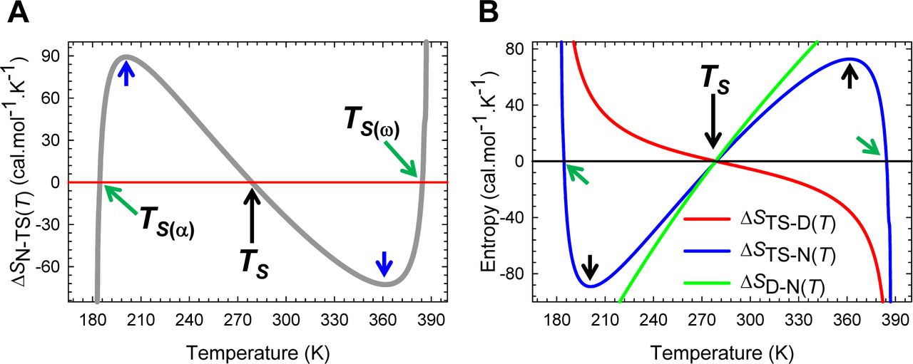
Substituting the expression for the temperature-dependence of GD-N(T) (Eq. (A3), Figure 1) in Eqs. (1) and (2) enables the temperature-dependence of the curve-crossing relative to the DSE and the NSE to be ascertained (Figure 2; substituted expressions not shown). Because by postulate the force constants, ΔCpD-N, and mD-N are temperature-invariant for any given primary sequence that folds in a two-state manner at constant pressure and solvent conditions, we get from inspection of Eqs. (1) and (2) that the discriminant φ, and  must be a maximum when ΔGD-N(T) is a maximum. Because ΔGD-N(T) is a maximum at TS (the temperature at which the entropy of unfolding at equilibrium, ΔSD-N(T), is zero),6 a corollary is that φ and
  must be a maximum at TS; and any deviation in the temperature from TS will only lead to their decrease. Consequently, mTS-D(T) and βT(fold)(T) (= mTS-D(T)/mD-N) are always a minimum, and mTS-N(T) and βT(unfold)(T) (= mTS-N(T)/mD-N) are always a maximum at TS. This gives rise to two further corollaries: Any deviation in the temperature from TS can only lead to: (i) an increase in mTS-D(T) and βT(fold)(T); and (ii) a decrease in mTS-N(T) and βT(unfold)(T) (Figure 2 and Figure 2−figure supplement 1). In other words, when T = TS, the TSE is the least native-like in terms of the SASA (solvent accessible surface area), and any deviation in temperature causes the TSE to become more native-like. A further consequence of mTS-D(T) being a minimum at TS is that if for a two-state-folding primary sequence there exists a chevron with a well-defined linear folding arm at TS, then mTS-D(T) > 0 and βT(fold)(T) > 0 for all temperatures (Figure 2A and Figure 2−figure supplement 1A). Since the curve-crossing is physically undefined for φ < 0 owing to there being no real roots, the maximum theoretically possible value of mTS-D(T) will occur when φ = 0 and is given by:
  where Tα and Tω are the temperature limits such that for T < Tα and T > Tω, a two-state system is not physically defined (see Paper II). Because mD-N = mTS-D(T) + mTS-N(T) for a two-state system, and mD-N is temperature-invariant by postulate, the theoretical minimum of mTS-N(T) is given by:
  . Now, since mTS-N(T) is a maximum and positive at TS but its minimum is negative, a consequence is that mTS-N(T) = βT(unfold)(T) = 0 at two unique temperatures, one in the ultralow (TS(α)) and the other in the high (TS(ω)) temperature regime, and negative for Tα ≤ T < TS(α) and TS(ω) < T ≤ Tω (Figure 2B and Figure 2−figure supplement 1B). Obviously, mTS-D(T) = mD-N and βT(fold)(T) is unity at TS(α) and TS(ω). To summarize, unlike mTS-D(T) and βT(fold)(T) which are positive for all temperatures and a minimum at TS, mTS-N(T) and βT(unfold)(T) are a maximum at TS, zero at TS(α) and TS(ω), and negative for Tα ≤ T < TS(α) and TS(ω) < T ≤ Tω.

(A) βT(fold)(T) is a minimum at TS, unity at TS(α) and TS(ω), and greater than unity for Tα ≤ T < TS(α) and TS(ω) < T ≤ Tω. The slope of this curve is given by  (B) βT(unfold)(T) is a maximum at TS, zero at TS(α) and TS(ω), and negative for Tα ≤ T < TS(α) and TS(ω) < T ≤ Tω. The slope of this curve is given by
  . From the perspective of Tanford’s framework, the SASA of the TSE is the least native-like at TS but becomes progressively more native-like as the temperature deviates from the TS, and is identical to the SASA of the NSE at TS(α) and TS(ω); and for Tα ≤ T < TS(α) and TS(ω) < T ≤ Tω, the TSE is more compact than the NSE.

(A) mTS-D(T) is a minimum at TS, is identical to mD-N at TS(α) and TS(ω), and is greater than mD-N for Tα ≤ T < TS(α) and TS(ω) < T ≤ Tω. The slope of this curve is given by  (B) mTS-N(T) is a maximum at TS, zero at TS(α) and TS(ω), and negative for Tα ≤ T < TS(α) and TS(ω) < T ≤ Tω. The slope of this curve is given by
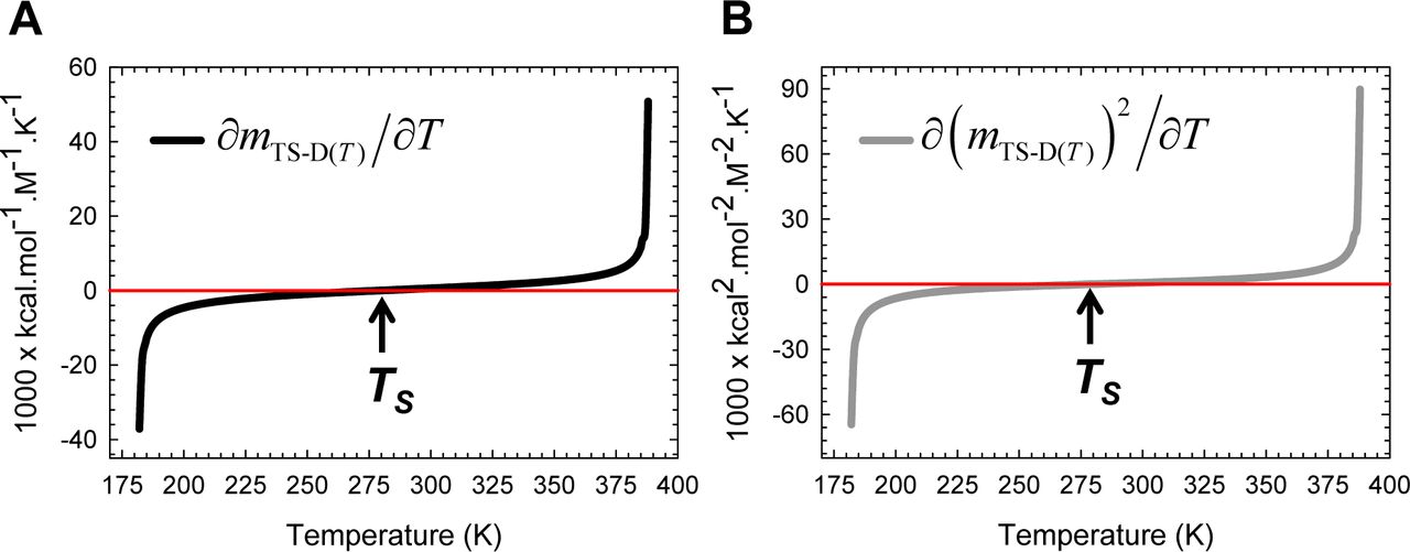
  . While the slopes of these curves are related to the activation entropies, the second derivatives of these functions with respect to temperature are related to the heat capacities of activation as shown in Paper-II. The values of the reference temperatures are given in Table 1.
The predicted Leffler-Hammond shift, which must be valid for any two-state system, is in agreement with the experimental data on the temperature-dependent behaviour of other two-state systems (Table 1 in Dimitriadis et al., 2004; Table 1 in Taskent et al., 2008; Fig. 5C in Otzen and Oliveberg, 2004),8-12 with the rate at which the curve-crossing shifts with stability (relative to the vertex of the DSE-parabola) being given by  . Importantly, just as the Leffler-Hammond movement is rationalized in physical organic chemistry using Marcus theory,13-15 we can similarly rationalize these effects in protein folding using parabolic approximation (Figures 3, 4, and Figure 4−figure supplement 1). When T = TS, ΔGTS-D(T) is a minimum, and ΔGD-N(T) and ΔGTS-N(T) are both a maximum; and any increase or decrease in the temperature relative to TS leads to a decrease in ΔGTS-N(T), and an increase in ΔGTS-D(T), consequently, leading to a decrease in ΔGD-N(T) (Figures 1, 3B and 5). Naturally at Tc and Tm, ΔGTS-D(T) = ΔGTS-N(T), kf(T) = ku(T), and ΔGD-N(T)= 0 (Figure 3C). The reason why mTS-D(T) = mD-N, and mTS-N(T) = 0 at TS(α) and TS(ω) is apparent from Figures 4A, 4C and Figure 4−figure supplement 1A: The right arm of the DSE-parabola intersects the vertex of the NSE-parabola leading to ΔGTS-D(T) = α(mTS-D(T))2 = α(mD-N)2 = λ, ΔGTS-N(T) = ω(mTS-N(T))2 = 0, and ΔGD-N(T) = − λ. Importantly, in contrast to unfolding which can become barrierless at TS(α) and TS(ω), folding is barrier-limited at all temperatures, with the absolute minimum of ΔGTS-D(T) occurring at TS; and any deviation in the temperature from TS will only lead to an increase in ΔGTS-D(T) (Figure 5A). Thus, a corollary is that if folding is barrier-limited at TS (i.e., the chevron has a well-defined linear folding arm with a finite slope at TS), then a protein that folds via two-state mechanism can never spontaneously (i.e., unaided by ligands, co-solvents etc.) switch to a downhill mechanism (Type 0 scenario according to the Energy Landscape Theory; see Fig. 6 in Onuchic et al., 1997), no matter what the temperature, and irrespective of how fast or slow it folds. Although unfolding is barrierless at TS(α) and TS(ω), it is once again barrier-limited for Tα ≤ T < TS(α) and TS(ω) < T ≤ Tω, with the curve-crossing occurring to the right of the vertex of the NSE-parabola (Figures 4A, 4B, Figure 4−figure supplement 1B and 5B), such that mTS-D(T) > mD-N, mTS-N(T) < 0, βT(fold)(T) > 1 and βT(unfold)(T) < 0 (Figure 2 and Figure 2−figure supplement 1).
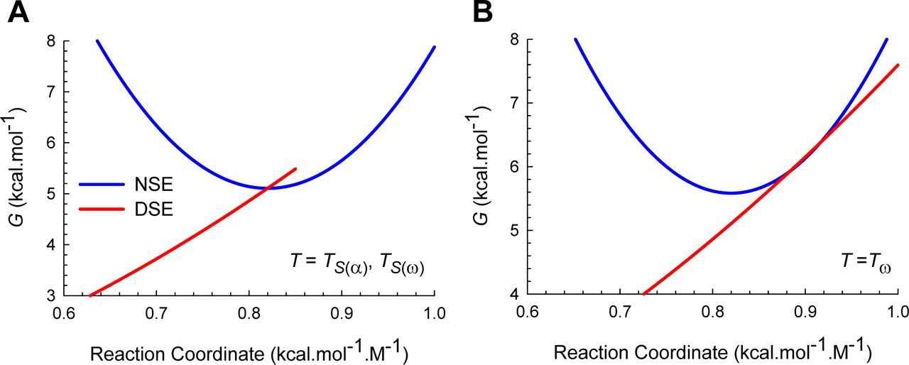
(A) Curve-crossing at TS(α) and TS(ω) where mTS-D(T) = mD-N, mTS-N(T) = 0, ΔGTS-N(T) = 0, ΔGTS-D(T) = α(mD-N)2 = λ, ΔGD-N(T) = − λ, and ku(T) = k0. (B) Curve-crossing at Tω where mTS-D(T) > mD-N.

(A) Figure 2A reproduced for comparison. (B) Curve-crossing at TS where ΔGD-N(T) is a maximum and purely enthalpic (Figure 1). The relevant parameters are as follows: ΔGTS-D(T) = 2.547 kcal.mol-1, ΔGTS-N(T) = 4.964 kcal.mol-1, ΔGD-N(T) = 2.417 kcal.mol-1, kf(T) = 22009 s-1, ku(T) = 280.8 s-1, mTS-D(T) = 0.5792 kcal.mol-1.M-1 and mTS-N(T) = 0.2408 kcal.mol-1.M-1. (C) Curve-crossing at Tm and Tc where ΔGTS-D(T) = ΔGTS-N(T) = 3.032 kcal.mol-1, ΔGD-N(T) = 0, kf(T) = ku(T) = 23618 s-1, mTS-D(T) = 0.6319 kcal.mol-1.M-1 and mTS-N(T) = 0.1881 kcal.mol-1.M-1.The DSE and the NSE-parabolas are given by GDSE(r,T)=αr2 and GNSE(r,T) = ω(mD-N − r)2 − ΔGD-N(T), respectively, α = 7.594 M2.mol.kcal-1, ω = 85.595 M2.mol.kcal-1, mD-N (0.82 kcal.mol-1.M-1) is the separation between the vertices of the DSE and the NSE-parabolas along the abscissa, and r is any point on the abscissa. The abscissae are identical for plots B and C. The values of the reference temperatures are given in Table 1.

(A) ΔGTS-D(T) is a minimum at TS, identical to λ = α(mD-N)2 = 5.106 kcal.mol-1 at TS(α) and TS(ω), and greater than λ for Tα ≤ T < TS(α) and TS(ω) < T ≤ Tω. Note that ∂ΔGTS-D(T)/∂T = −ΔSTS-D(T) = 0 at TS. (B) In contrast to ΔGTS-D(T) which has only one extremum, ΔGTS-N(T) is a maximum at TS and a minimum (zero) at TS(α) and TS(ω); consequently, ∂ΔGTS-N(T)/∂T = −∂STS-N(T) = 0 at TS(α), TS and TS(ω). Although unfolding is barrierless at TS(α) and TS(ω), it is once again barrier-limited for Tα ≤ T < TS(α) and TS(ω) < T ≤ Tω; however, unlike the conventional barrier-limited unfolding which is characteristic for TS(α) < T < TS(ω), these two regimes fall under the Marcus-inverted-region and can be rationalized from Figures 2, 4, and their figure supplements. The values of the reference temperatures are given in Table 1.

(A) kf(T) is a maximum and ΔHTS-D(T)= 0 at TH(TS-D). The slope of this curve is given by −ΔHTS-D(T)/R. (B) Unlike kf(T) which has only one extremum, ku(T) is a minimum at TH(TS-N) and a maximum at TS(α) and TS(ω). Consequently, ΔHTS-N(T) = 0 at TS(α), TH(TS-N) and TS(ω). The slope of this curve is given by −ΔHTS-N(T)/R. When T = TS(α) or TS(ω), we have a unique scenario: mTS-N(T) = ΔGTS-N(T) = ΔHTS-N(T) = 0 ⇒ ΔSTS-N(T) = 0, and ku(T) = k0. Although unfolding is barrier-limited for Tα ≤ T < TS(α) and TS(ω) < T ≤ Tω, leading to ku(T) < k0, these ultra-low and high temperature regimes fall under the Marcus-inverted-regime as compared to the conventional barrier-limited unfolding which is characteristic for TS(α) < T < TS(ω) (the curve-crossing occurs in-between the vertices of the DSE and the NSE Gibbs basins) and can be rationalized comprehensively when considered in conjunction with Figures 2, 4, and 5 (see also their figure supplements if any). The maxima of kf(T) and ku(T), as well as the inverted-region can be better appreciated on a linear scale as shown in the figure supplement. The values of the reference temperatures are given in Table 1.

(A) kobs(T) is a maximum at TS(α) and TS(ω), and a minimum around Tc (blue pointer). The red pointer indicates Tm. The steep increase in kobs(T) at very low and high temperatures is due to ΔGTS-N(T) approaching zero as described in previous figures. (B) An overlay of kf(T), ku(T) and kobs(T) to illuminate how the features of kobs(T) arise from the sum of kf(T) and ku(T). The slopes of the red and blue curves are given by ∆HTS-D(T)/RT2 and ∆HTS-N(T)/RT2, respectively.
To summarize, for any two-state folder, unfolding is conventional barrier-limited for TS(α) < T < TS(ω) and the position of the TSE or the curve-crossing occurs in between the vertices of the DSE and the NSE parabolas. As the temperature deviates from TS, the SASA of the TSE becomes progressively native-like, with a concomitant increase and a decrease in ΔGTS-D(T) and ΔGTS-N(T), respectively. When T = TS(α) and TS(ω), the curve-crossing occurs precisely at the vertex of the NSE-parabola, the SASA of the TSE is identical to that of the NSE, and unfolding is barrierless; and for Tα ≤ T < TSα and TS(ω) < T ≤ Tω, unfolding is once again barrier-limited but falls under the Marcus-inverted-regime with the curve-crossing occurring on the right-arm of the NSE-parabola, leading to the SASA of the NSE being greater than that of the TSE (i.e., the TSE is more compact than the NSE). Importantly, for T < Tα and T > Tω, the TSE cannot be physically defined owing to  being mathematically undefined for φ > 0. A consequence is that kf(T) and ku(T) become physically undefined, leading to ΔGD-N(T) = RT ln (kf(T)/ku(T)) being physically undefined, such that all of the conformers will be confined to a single Gibbs energy well, which is the DSE, and the protein will cease to function.16 Thus, from the view point of the physics of phase transitions, Tα ≤ T ≤ Tω denotes the coexistence temperature-range where the DSE and the NSE, which are in a dynamic equilibrium, will coexist as two distinct phases; and for T < Tα and T > Tω there will be a single phase, which is the DSE, with Tα and Tω being the limiting temperatures for coexistence, or phase boundary temperatures from the view point of the DSE.17-23 This is roughly analogous to the operating temperature range of a logic circuit such as a microprocessor; and just as this range is a function of its constituent material, the physically definable temperature range of a two-state system is a function of the primary sequence when pressure and solvent are constant, and importantly, can be modulated by a variety of cis-acting and trans-acting factors (see Paper-I). The limit of equilibrium stability below which a two-state system becomes physically undefined is given by: ΔGD-N(T)|T = Tα, Tω = −λω/(ω − α). Consequently, the physically meaningful range of equilibrium stability for a two-state system is given by: ΔGD-N(TS) + [λω/(ω − α)], where ΔGD-N(TS) is the stability at TS and is apparent from inspection of Figure 5−figure supplement 1. This is akin to the stability range over which Marcus theory is physically realistic (see Kresge, 1973, page 494).24

(A) The stability of a two-state system at constant pressure and solvent conditions is the greatest when the denatured conformers are displaced the least from the mean of their ensemble along the SASA-RC to reach the TSE. The length of the green dotted line is identical to ΔGD-N(Ts) + [ λω/(ω-α)], where ΔGD-N(TS) is the stability at TS. The slope of this curve equals  . (B) ΔGD-N(T) will be the greatest when the native conformers expose the greatest amount of SASA to reach the TSE. The slope of this curve equals
  .
.
Because by postulate mD-N, mTS-D(T) and mTS-N(T) are true proxies for ΔSASAD-N, ΔSASAD-TS(T) and ΔSASATS-N(T), respectively (see Paper I), we have three fundamentally important corollaries that must hold for all two-state systems at constant pressure and solvent conditions: (i) the Gibbs barrier to folding is the least when the denatured conformers bury the least amount of SASA to reach the TSE (Figure 5−figure supplement 2A); (ii) the Gibbs barrier to unfolding is the greatest when the native conformers expose the greatest amount of SASA to reach the TSE (Figure 5−figure supplement 2B); and (iii) equilibrium stability is the greatest when the conformers in the DSE are displaced the least from the mean of their ensemble along the SASA-RC to reach the TSE (the principle of least displacement; Figure 5−figure supplement 1).

(A) ΔGTS-D(T) is the least when the denatured conformers bury the least amount of SASA to reach the TSE. The slope of this curve equals 2λβT(fold)(T). (B) ΔGTS-N(T) is the greatest when the native conformers expose the greatest amount of SASA to reach the TSE. The green pointer indicates TS(α) and TS(ω) where mTS-D(T) = mD-N, mTS-N(T) = βT(unfold)(T) = 0, ΔGTS-N(T) = 0, ΔGTS-D(T) = α(mD-N)2 = λ, and ΔGD-N(T) = − λ. The slope of this curve equals 2ωmTS-N(T)mD-N. Because mTS-N(T) < 0 for Tα ≤ T < TS(α) and TS(ω) < T ≤ Tω, the slope is negative for the part that is to the left of the green pointer.
Temperature-dependence of the folding, unfolding, and the observed rate constants
Inspection of Figures 6A and Figure 6−figure supplement 1A demonstrates that Eq. (5) makes a remarkable prediction that kf(T) has a non-linear dependence on temperature. Starting from the lowest temperature (Tα) at which a two-state system is physically defined, kf(T) initially increases with an increase in the temperature and reaches a maximal value at T = TH(TS-D) where ∂ ln kf(T)/∂T = ΔHTS-D(T)/RT2 = 0; and any further increase in temperature beyond this point will cause a decrease in kf(T) until the temperature Tω is reached, such that for T > Tω, kf(T) is undefined. Inspection of Figures 6B and Figure 6−figure supplement 1B demonstrates that the temperature-dependence of ku(T) is far more complex: Starting from Tα, ku(T) increases with temperature for the regime Tα ≤ T < TS(α) (the low-temperature Marcus-inverted-regime), reaches a maximum when T = TS(α) (ku(T) = k0; the first extremum of ku(T)), and decreases with further rise in temperature for the regime TS(α) < T < TH(TS-N) such that when T = TH(TS-N), ku(T) is a minimum (the second extremum of ku(T)). And for TH(TS-N) < T < TS(ω), an increase in temperature will lead to an increase in ku(T), eventually leading to its saturation at T = TS(ω) (ku(T) = k0; the third extremum of ku(T)), and decreases with further rise in temperature for TS(ω) < T ≤ Tω (the high-temperature Marcus-inverted-regime). Thus, in contrast to kf(T) which has only one extremum, ku(T) is characterised by three extrema where ∂ ln ku(T)/∂T = ΔHTS-N(T)/R2 = 0, and may be rationalized from the temperature-dependence of mTS-D(T) and mTS-N(T), the Gibbs barrier heights for folding and unfolding, and the intersection of the DSE and the NSE Gibbs parabolas (Figures 2-5 and their figure supplements). We will show in subsequent publications that the inverted behaviour at very low and high temperatures is not common to all fixed two-state systems and depends on the mean and variance of the Gaussian distribution of the SASA of the conformers in the DSE and the NSE.

(A) kf(T) is a maximum and ΔHTS-D(T) = 0 at TH(TS-D). The slope of this curve is given by kf(T)∆HTS-D(T)/RT2. (B) Unlike kf(T) which has only one extremum, ku(T) is a minimum at TH(TS-N) and a maximum at TS(α) and TS(ω). Although the minimum of ku(T) is not apparent on a linear scale, the barrierless and inverted-regimes for unfolding are readily apparent. The slope of this curve is given by ku(T)∆HTS-N(T)/RT2. The features of these curves arise primarily from the temperature-dependence of the equilibrium constants for the partial folding (D ⇌ [TS]) and unfolding (N ⇌ [TS]) reactions as shown later. The green dots represent TS.
Since the ultimate test of any hypothesis is experiment, the most important question now is how well do the calculated rate constants compare with experiment? Although Nguyen et al. have investigated the non-Arrhenius behaviour of the FBP28 WW, they find that the behaviour of its wild type is erratic, with its folding being three-state for T < Tm and two-state for T > Tm (Fig. 3A in Nguyen et al., 2003). Consequently, non-Arrhenius data for the wild type FBP28 WW are lacking. Incidentally, this atypical behaviour is probably artefactual since the protein aggregates and forms fibrils under the experimental conditions in which the measurements were made (see Figs. 2, 3 and 6 in Ferguson et al., 2003).25,26 Nevertheless, data for ΔNΔC Y11R W30F, a variant of FBP28 WW are available between ∽ 298 and ∽357 K (Fig. 4A in Nguyen et al., 2003). Now since the relaxation time constants for the fast phase of wild type FBP28 WW (∽ 30 μs at 39.5 °C and < 15 μs at 65 °C, page 3950, Fig. 3A, Nguyen et al., 2003) are very similar to those of ΔNΔC Y11R W30F (∽ 28 μs at 40 °C and 11 μs at 65 °C, page 3952), a reasonable approximation is that the temperature-dependence of kf(T) and ku(T) of the wild type and the mutant must be similar. Consequently, the temperature-dependence of the rate constants for the wild type FBP28 WW calculated using parabolic approximation must be very similar to the data for ΔNΔC Y11R W30F reported by Nguyen et al. The remarkable agreement between the said datasets is readily apparent from a comparison of Fig. 4A of Nguyen et al., and Figure 6−figure supplement 2, and serves an important test of the hypothesis.

A combined and appropriately rescaled version of Figure 6 to enable a ready comparison of the rate constants for FBP28 WW wild type (calculated using parabolic approximation) and the experimental rate constants for ΔNΔC Y11R W30F, a variant of FBP28 WW (reported by Nguyen et al., 2003, Fig. 4A). Note that the intersection of kf(T) and ku(T) is shifted to the left along the abscissa for the wild type FBP28 WW since its Tm is ∽ 10 K greater than that of ΔNΔC Y11R W30F (see Table 1 in Nguyen et al., 2003).25
Since the temperature-dependence of kf(T) and ku(T) across a wide temperature range is known, the variation in the observed rate constant (kobs(T)) with temperature may be readily ascertained using (see Appendix)

Inspection of Figure 7 demonstrates that ln(kobs(T)) vs temperature is a smooth ‘W-shaped’ curve, with kobs(T) being dominated by kf(T) around TH(TS-N), and by ku(T) for T < Tc and T > Tm, which is precisely why the kinks in ln(kobs(T)) occur around these temperatures. It is easy to see that at Tc or Tm, kf(T) = ku(T) ⇒ kobs(T) = 2kf(T) = 2ku(T), ΔGD-N(T) = RT ln (kf(T)/ku(T))) = 0 or ΔGTS-D(T) = ΔGTS-N(T) (Figures 3C and Figure 7−figure supplement 1). In other words, for a two-state system, Tc and Tm determined at equilibrium must be identical to the temperatures at which kf(T) and ku(T) intersect. This is a consequence of the principle of microscopic reversibility, i.e., the equilibrium and kinetic stabilities must be identical for a two-state system at all temperatures.27 It is precisely for this reason that the value of the prefactor in the Arrhenius expressions for the rate constants must be identical for both the folding and the unfolding reactions at all temperatures (Eqs. (5) and (6)). The steep increase in kobs(T) for T < Tc and T > Tm is due to the ΔGTS-N(T) approaching zero as described earlier. The argument that the shapes of the curves must be conserved across two-state systems applies not only to the temperature-dependence of mTS-D(T), mTS-N(T), ΔGTS-D(T) and ΔGTS-N(T) described so far, but to the rest of the state functions that will be described in this article (see Paper-I).

(A) kf(T) is a maximum at TH(TS-D) and ku(T) is a minimum at TH(TS-N). The slopes of the black and grey curves are given by ∆HTS-D(T)/RT2 and ∆HTS-N(T)/RT2, respectively. (B) ΔGTS-D(T) and ΔGTS-N(T) are a minimum and a maximum, respectively, at TS (red pointers) leading to ΔGD-N(T) being a maximum at TS (Figure 1). Equilibrium stability is thus a consequence or the equilibrium manifestation of the underlying kinetic behaviour. The rate constants are identical at Tc and Tm, leading to ∆GD-N(T)=RT ln (kf(T)/ku(T))=∆GTS-N(T)-∆GTS-D(T)=0.
An important conclusion that we may draw from these data is the following: Because we have assumed a temperature-invariant prefactor and yet find that the kinetics are non-Arrhenius, it essentially implies that one does not need to invoke a super-Arrhenius temperature-dependence of the configurational diffusion constant to explain the non-Arrhenius behaviour of proteins.28-32 Instead, as long as the enthalpies and the entropies of unfolding/folding at equilibrium display a large variation with temperature, and equilibrium stability is a non-linear function of temperature, both kf(T) and ku(T) will have a non-linear dependence on temperature. This leads to two corollaries: (i) since the large variation in equilibrium enthalpies and entropies of unfolding, including the pronounced curvature in ΔGD-N(T) of proteins with temperature is due to the large and positive ΔCpD-N, “non-Arrhenius kinetics can be particularly acute for reactions that are accompanied by large changes in the heat capacity”; and (ii) because the change in heat capacity upon unfolding is, to a first approximation, proportional to the change in SASA that accompanies it, and since the change in SASA upon unfolding/folding increases with chain-length,33,34 “non-Arrhenius kinetics, in general, can be particularly pronounced for large proteins, as compared to very small proteins and peptides.”
Temperature-dependence of activation enthalpies
Inspection of Figure 8 demonstrates that for the partial folding reaction D ⇌ [TS]: (i) ΔHTS-D(T) > 0 for Tα ≤ T < TH(TS-D); (ii) ΔHTS-D(T) < 0 for TH(TS-D) < T ≤ Tω and (iii) ΔHTS-D(T) = 0 for T = TH(TS-D). Thus, the activation of the denatured conformers to the TSE is enthalpically: (i) unfavourable for Tα ≤ T < TH(TS-D); (ii) favourable for TH(TS-D) < T ≤ Tω; and (iii) neutral when T = TH(TS-D). Consequently, at TH(TS-D), ΔGTS-D(T) is purely due to the difference in entropy between the DSE and the TSE (ΔGTS-D(T) = −TΔSTS-D(T)) with kf(T) being given by

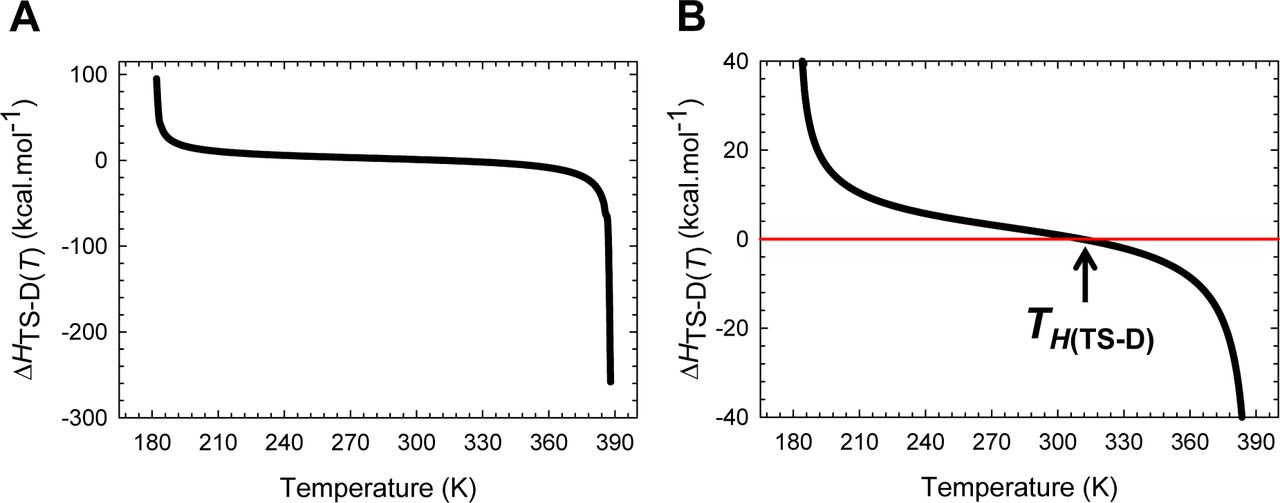
(A) The variation in ΔHTS-D(T) function with temperature. The slope of this curve varies with temperature, equals ΔCpTS-D(T), and is algebraically negative. (B) An appropriately scaled version of the plot on the left to illuminate the three important scenarios: (i) ΔHTS-D(T) > 0 for Tα ≤ T < TH(TS-D); (ii) ΔHTS-D(T) < 0 for TH(TS-D) < T ≤ Tω; and (iii) ΔHTS-D(T) = 0 when T = TH(TS-D). Note that kf(T) is a maximum at TH(TS-D).
Because kf(T) is a maximum at TH(TS-D) (∂ ln kf(T)/∂T = 0), a corollary is that “for a two-state folder at constant pressure and solvent conditions, if the prefactor is temperature-invariant, then kf(T) will be a maximum when the Gibbs barrier to folding is purely entropic.” This statement is valid only if the prefactor is temperature-invariant. Now since ΔGTS-D(T) > 0 for all temperatures (Figure 5A and Table 1), it is imperative that ΔSTS-D(T) < 0 at TH(TS-D) (see activation entropy for folding).
Unlike the ΔHTS-D(T) function which changes its algebraic sign only once across the entire temperature range over which a two-state system is physically defined, the behaviour of ΔHTS-N(T) function is far more complex (Figure 9): (i) ΔHTS-N(T) > 0 for Tα ≤ T < TS(α) and TH(TS-N) < T < TS(ω); (ii) ΔHTS-N(T) < 0 for TS(α) < T < TH(TS-N) and TS(ω) < T ≤ Tω; and (iii) ΔHTS-N(T) = 0 at TS(α), TH(TS-N), and TS(ω). Consequently, we may state that the activation of native conformers to the TSE is enthalpically: (i) unfavourable for Tα ≤ T < TS(α) and TH(TS-N) < T < TS(ω); (ii) favourable for TS(α) < T < TH(TS-N) and TS(ω) < T ≤ Tω; and (iii) neutral at TS(α), TH(TS-N), and TS(ω). If we reverse the reaction-direction, the algebraic signs invert leading to a change in the interpretation. Thus, for the partial folding reaction [TS] ⇌ N, the flux of the conformers from the TSE to the NSE is enthalpically: (i) favourable for Tα ≤ T < TS(α) and TH(TS-N) < T < TS(ω) (ΔHN-TS(T) < 0); (ii) unfavourable for TS(α) < T < TH(TS-N) and TS(ω) < T ≤ Tω (ΔHN-TS(T) > 0); and (iii) neither favourable nor unfavourable at TS(α), TH(TS-N), and TS(ω) (Figure 9−figure supplement 1A). Note that the term “flux” implies “diffusion of the conformers from one reaction state to the other on the Gibbs energy surface,” and as such is an “operational definition.”
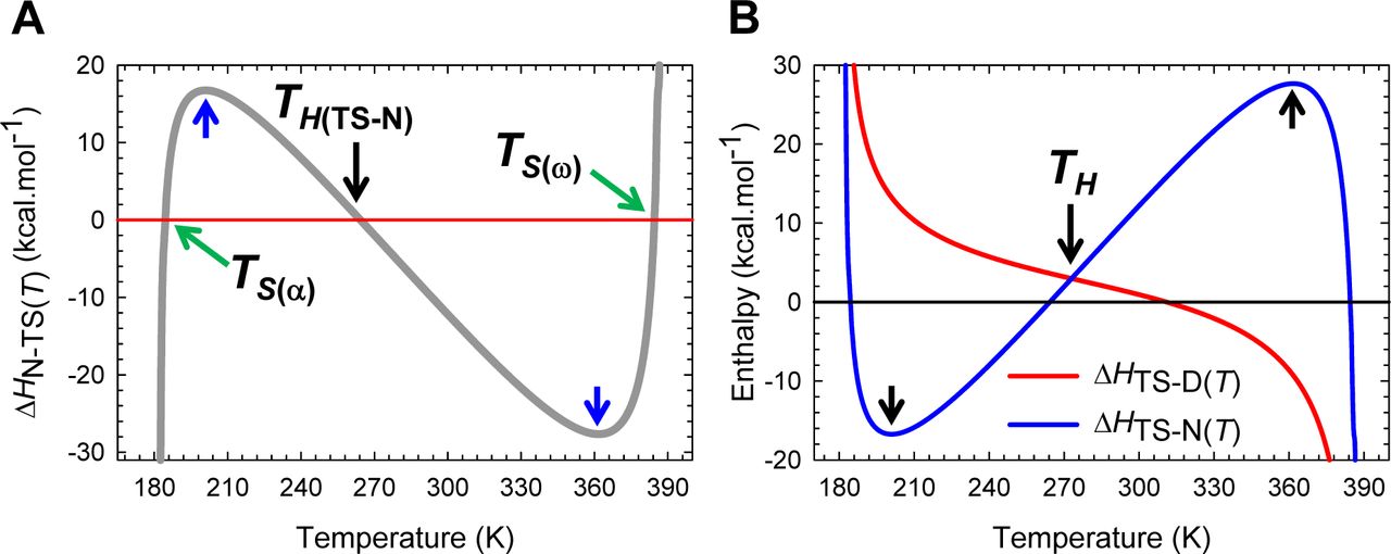
(A) An appropriately scaled view of the change in enthalpy for the partial folding reaction [TS] ⇌ N. The flux of the conformers from the TSE to the NSE is enthalpically: (i) favourable for Tα ≤ T < TS(α) and TH(TS-N) < T < TS(ω) (ΔHN-TS(T) < 0); (ii) unfavourable for TS(α) < T < TH(TS-N) and TS(ω) < T ≤ Tω (ΔHN-TS(T) > 0); and (iii) neither favourable nor unfavourable at TS(α), TH(TS-N), and TS(ω). The blue pointers indicate the temperatures where ΔCpN-TS(T) (or −ΔCpTS-N(T)) is zero. (B) The intersection of the ΔHTS-D(T) and ΔHTS-N(T) functions occurs precisely at TH. The requirement that both ΔHTS-D(T) and ΔHTS-N(T) be positive at the point of intersection is a consequence of the theoretical relationship: TH(TS-N) < TH < TS < TH(TS-D) and must be satisfied by all two-state systems (see Paper II). Note that the net flux of the conformers from the DSE to the NSE at TH is driven purely by entropy (ΔGD-N(T) = –T ΔSD-N(T)).

(A) The variation in ΔHTS-N(T) function with temperature. The slope of this curve equals ΔCpTS-N(T) and is zero at TCpTS-N(α) and TCpTS-N(ω). (B) An appropriately scaled version of the figure on the left to illuminate the various temperature-regimes and their implications: (i) ΔHTS-N(T) > 0 for Tα ≤ T < TS(α) and TH(TS-N) < T < TS(ω); (ii) ΔHTS-N(T) < 0 for TS(α) < T < TH(TS-N) and TS(ω) < T ≤ Tω; and (iii) ΔHTS-N(T) = 0 at TS(α), TH(TS-N), and TS(ω). Note that at TS(α) and TS(ω), we have the unique scenario: mTS-N(T) = ΔGTS-N(T) = ΔSTS-N(T) = ΔHTS-N(T) = 0, and ku(T) = k0. The values of the reference temperatures are given in Table 1.
Importantly, although ∂ ln ku(T)/∂T = 0 ⇒ ΔHTS-N(T) = 0 at TS(α), TH(TS-N), and TS(ω), the behaviour of the system at TS(α) and TS(ω) is distinctly different from that at TH(TS-N): While mTS-N(T) = ΔGTS-N(T) = ΔHTS-N(T) = ΔSTS-N(T) = 0, mTS-D(T) = mD-N, ΔGTS-D(T) = ΔGN-D(T) = λ, and ku(T) = k0 at TS(α) and TS(ω) (note that if both ΔGTS-N(T) and ΔHTS-N(T) are zero, then ΔSTS-N(T) must also be zero, see activation entropies), ku(T) is a minimum (ku(T) ≪ k0) with the Gibbs barrier to unfolding being purely entropic (ΔGTS-N(T) = −TΔSTS-N(T)) at TH(TS-N). Consequently, we may write

Thus, a corollary is that “for two-state system at constant pressure and solvent conditions, if the prefactor is temperature-invariant, then ku(T) will be a minimum when the Gibbs barrier to unfolding is purely entropic.” Since ΔGTS-N(T) > 0 at TH(TS-N) (Figure 5B and Table 1), it is imperative that ΔSTS-N(T) be negative at TH(TS-N) (see activation entropy for unfolding).
The criteria for two-state folding from the viewpoint of enthalpy are the following: (i) the condition that ΔHD-N(T) = ΔHTS-N(T) − ΔHTS-D(T) must be satisfied at all temperatures; (ii) the intersection of ΔHTS-D(T) and ΔHTS-N(T) functions calculated directly from the temperature-dependence of the experimentally determined kf(T) and ku(T), respectively, must be identical to the independently estimated TH from equilibrium thermal denaturation experiments; and (iii) the condition that TH(TS-N) < TH < TS < TH(TS-D) must be satisfied. A corollary of the last statement is that both ΔHTS-D(T) and ΔHTS-N(T) functions must be positive at the point of intersection. These aspects are readily apparent from Figure 9−figure supplement 1B and Figure 9−figure supplement 2.

(A) ΔHD-N(T) for the reaction N ⇌ D is zero at the temperature where ΔHTS-D(T) and ΔHTS-N(T) functions intersect (the intersection of green curve and zero reference line must align vertically with the point where the blue and the red curves intersect). The intersection of ΔHD-N(T) and ΔHTS-N(T) functions (green and blue curves) occurs precisely when T = TH(TS-D). This is expected since ΔHTS-D(T) = 0 at TH(TS-D). The similarity in the slopes of the ΔHD-N(T) and ΔHTS-N(T) functions between ∽ 240 K and ∽ 320 K implies that most of ΔCpD-N stems from the first-half of the unfolding reaction N ⇌ [TS]. (B) An appropriately scaled view of the encircled area in the figure on the left. When T = TH(TS-N), ΔHTS-D(T) is identical to |ΔHD-N(T)| or ΔHN-D(T). Further, at the temperature where ΔHTS-D(T) and ΔHD-N(T) functions intersect (i.e., the intersection of the red and the green curves), the absolute enthalpy of the DSE (HD(T)) is exactly half the algebraic sum of the absolute enthalpies of the TSE (HTS(T)) and the NSE (HN(T)), i.e., HD(T) = (HTS(T)+HN(T))/2. The various auxiliary relationships that may obtained from the intersection of various state functions are addressed in subsequent publications.
Temperature-dependence of activation entropies
Inspection of Figure 10 shows that for the partial folding reaction D ⇌ [TS], ΔSTS-D(T) which is positive at low temperature, decreases in magnitude with an increase in temperature and becomes zero at TS, where the SASA of the TSE is the least native-like, ΔGTS-D(T) is a minimum (∂ΔGTS-D(T)/∂T = −ΔSTS-D(T) = 0) and ΔGD-N(T) is a maximum (∂ΔGD-N(T)/∂T = −ΔSD-N(T) = 0; Figures 1, 2, 5A, Figure 10−figure supplements 1 and 2); and any further increase in temperature beyond this point causes ΔSTS-D(T) to become negative. Thus, the activation of denatured conformers to the TSE is entropically: (i) favourable for Tα ≤ T < TS; (ii) unfavourable for TS < T ≤ Tω; and (iii) neutral when T = TS. At TS the Gibbs barrier to folding is purely due to the difference in enthalpy between the DSE and the TSE with kf(T) being given by


(A) ΔSTS-D(T) is zero when the denatured conformers are displaced the least from the mean of their ensemble to reach the TSE along the SASA-RC. The slope of this curve is given by  (B) ΔSTS-D(T) is zero when the SASA of the TSE is the least native-like. The slope of this curve is given by
  . The blue and the red sections of the curves represent the temperature regimes Tα ≤ T ≤ TS and TS ≤ T ≤ Tω, respectively.
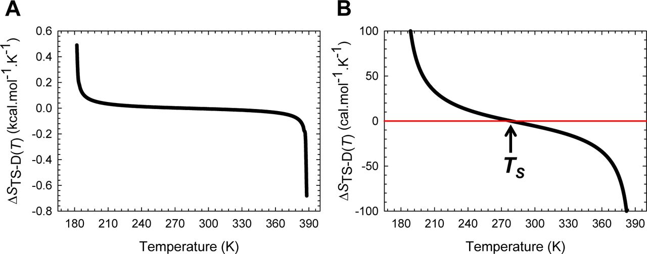
(A) The variation in ΔSTS-D(T) function with temperature. The slope of this curve varies with temperature and equals ΔCpTS-D(T)/T. (B) An appropriately scaled version of the figure on the left to illuminate the three temperature regimes and their implications: (i) ΔSTS-D(T) > 0 for Tα ≤ T < TS; (ii) ΔSTS-D(T) < 0 for TS < T ≤ Tω; and (iii) ΔSTS-D(T) = 0 when T = TS.
Inspection of Figure 11 demonstrates that the behaviour of the ΔSTS-N(T) function is far more complex than the ΔSTS-D(T) function: (i) ΔSTS-N(T) > 0 for Tα ≤ T < TS(α) and TS < T < TS(ω); (ii) ΔSTS-N(T) < 0 for TS(α) < T < TS and TS(ω) < T ≤ Tω; and (iii) ΔSTS-N(T) = 0 at TS(α), TS, and TS(ω). Consequently, we may state that the activation of native conformers to the TSE is entropically: (i) favourable for Tα ≤ T < TS(α) and TS < T < TS(ω); (ii) unfavourable for TS(α) < T < TS and TS(ω) < T ≤ Tω; and (iii) neutral at TS(α), TS, and TS(ω). If we reverse the reaction-direction (Figure 11−figure supplement 1A), the algebraic signs invert leading to a change in the interpretation. Consequently, we may state that for the partial folding reaction [TS] ⇌ N, the flux of the conformers from the TSE to the NSE is entropically: (i) unfavourable for Tα ≤ T < TS(α) and TS < T < TS(ω) (ΔSN-TS(T) < 0); (ii) favourable for TS(α) < T < TS and TS(ω) < T ≤ Tω (ΔSN-TS(T) > 0); and (iii) neutral at TS(α), TS, and TS(ω).

(A) ΔGTS-D(T) is always the least when it is purely enthalpic. The slope of this curve equals-TΔSTS-D(T)/ΔCpTS-D(T). (B) The stability is always the greatest when the activation entropy for folding is the zero. The slope of this curve equals-TΔSTS-D(T)/ΔCpTS-D(T). The blue and the red sections of the curves represent the temperature regimes Tα ≤ T ≤ TS and TS ≤ T ≤ Tω, respectively.
(A) An appropriately scaled view of the change in entropy for the partial folding reaction [TS] ⇌ N. The slope of this curve equals ΔCpN-TS(T)/T (or −ΔCpN-TS(T)/T and is zero at TCpTS-N(α) and TCpTS-N(ω). The flux of the conformers from the TSE to the NSE is entropically: (i) unfavourable for Tα ≤ T < TS(α) and TS < T < TS(ω) (ΔSN-TS(T) < 0); (ii) favourable for TS(α) < T < TS and TS(ω) < T ≤ Tω (ΔSN-TS(T) > 0); and (iii) neutral at TS(α), TS, and TS(ω). (B) An overlay of ΔSD-N(T), ΔSTS-D(T) and ΔSTS-N(T) functions. Unlike the ΔHTS-D(T) and ΔHTS-N(T) functions which must be positive at the point of intersection (Figure 9−figure supplement 1B), theory dictates that both ΔSTS-D(T) and ΔSTS-N(T) functions must independently be equal to zero at TS, leading to the unique scenario: SD(T) = STS(T) = SN(T). The similarity in the slopes of the ΔSDN(T) and ΔSTS-N(T) functions between ∽ 240 K and ∽ 320 K implies that most of ΔCpD-N stems from the first-half of the unfolding reaction N ⇌ [TS]. Consequently at TS, ΔGD-N(T) = ΔHDN(T), i.e., the net flux of the conformers from the DSE to the NSE is driven purely by enthalpy.

(A) The variation in ΔSTS-N(T) function with temperature. The slope of this curve, given by ΔCpTS-N(T)/T, varies with temperature, and is zero at TCpTS-N(α) and TCpTS-N(ω). (B) An appropriately scaled version of the figure on the left to illuminate the temperature regimes and their implications: (i) ΔSTS-N(T) > 0 for Tα ≤ T < TS(α) and TS < T < TS(ω); (ii) ΔSTS-N(T) < 0 for TS(α) < T < TS and TS(ω) < T ≤ Tω; and (iii) ΔSTS-N(T) = 0 at TS(α), TS, and TS(ω). Note that at TS(α) and TS(ω), we have the unique scenario: mTS-N(T) = ΔGTS-N(T) = ΔSTS-N(T) = ΔHTS-N(T) = 0, and ku(T) = k0. The values of the reference temperatures are given in Table 1.
At T = TS, the Gibbs barrier to unfolding is purely due to the difference in enthalpy between the TSE and the NSE (ΔGTS-N(T) = ΔHTS-N(T)) with ku(T) being given by

Although ΔSTS-N(T) = 0 ⇒ STS(T) = SN(T) at TS(α), TS, and TS(ω), the underlying thermodynamics is fundamentally different at TS as compared to TS(α) and TS(ω). While both ΔGTS-N(T) and mTS-N(T) are positive and a maximum, and ΔGTS-N(T) is purely enthalpic at TS (ΔGTS-N(T) = ΔHTS-N(T)), at TS(α) and TS(ω) we have mTS-N(T) = 0 ⇒ ΔGTS-N(T) = ω(mTS-N(T)2 = 0 ⇒ ΔHTS-N(T) = 0, and ΔGN-D(T) = ΔGTS-D(T) = λ; and because ΔGTS-N(T) = 0 at TS(α) and TS(ω), the rate constant for unfolding will reach an absolute maximum for that particular solvent and pressure at these two temperatures. To summarize, while at TS we have GTS(T) ≫ GN(T), SD(T) = STS(T) = SN(T), and ku(T) ≪ k0, when T = TS(α) and TS(ω), we have GTS(T) = GN(T), HTS(T) = HN(T), STS(T) = SN(T), and ku(T) = k0 (Figure 11−figure supplements 2 and 3). Thus, a fundamentally important conclusion that we may draw from these relationships is that “if two reaction-states on the folding pathway of a two-state system have identical SASA and Gibbs energy under identical environmental conditions, then their absolute enthalpies and entropies must be identical.” This must hold irrespective of whether or not the two reaction-states have identical, similar or dissimilar structures. We will revisit this scenario when we discuss the heat capacities of activation and the inapplicability of the Hammond postulate to protein folding reactions.

(A) Unlike the ΔSTS-D(T) function which is zero only once, ΔSTS-N(T) is zero once when the native conformers are displaced the greatest to reach the TSE (TS), and twice when this displacement is zero (green pointer; TS(α) and TS(ω)). The slope of this curve is given by  . (B) ΔSTS-N(T) is zero once when the difference in SASA between the TSE and the NSE is the greatest (TS), and twice when the SASA of the TSE is identical to that of the NSE (green pointer; TS(α) and TS(ω)). The slope of this curve is given by
  . The blue and the red sections of the curves represent the temperature regimes Tα ≤ T ≤ TS and TS ≤ T ≤ Tω, respectively.
The criteria for two-state folding from the viewpoint of entropy are the following: (i) the condition that ΔSD-N(T) = ΔSTS-N(T) — ΔSTS-D(T) must be satisfied at all temperatures; (ii) the intersection of ΔSTS-D(T) and ΔSTS-N(T) functions calculated directly from the slopes of the temperature-dependent shift in the curve-crossing relative to the DSE and the NSE, respectively, must be identical to the independently estimated TS from equilibrium thermal denaturation experiments (Figure 11−figure supplements 1B, 4 and 5); and (iii) both ΔSTS-D(T) and ΔSTS-N(T) functions must independently be equal to zero at TS.
Temperature-dependence of the Gibbs activation energies
Although the general features of the temperature-dependence of ΔGTS-D(T) and ΔGTS-N(T) were described earlier (Figure 5 and its figure supplements), it is instructive to discuss the same in terms of their constituent enthalpies and entropies.
The determinants of ΔGTS-D(T) in terms of its activation enthalpy and entropy may be readily deduced by partitioning the entire temperature range over which the two-state system is physically defined (Tα ≤ T ≤ Tω) into three distinct regimes using four unique reference temperatures: Tα, TS, TH(TS-D), and Tω (Figure 12 and Figure 12−figure supplement 1). (1) For Tα ≤ T < TS, the activation of conformers from the DSE to the TSE is entropically favoured (TΔSTS-D(T) > 0) but is more than offset by the endothermic activation enthalpy (ΔHTS-D(T) > 0), leading to incomplete compensation and a positive ΔGTS-D(T) (ΔHTS-D(T) – TΔSTS-D(T). When T = TS, ΔGTS-D(T) is a minimum (its lone extremum), and is purely due to the endothermic enthalpy of activation (ΔGTS-D(T) = ΔHTS-D(T) > 0. (2) For TS < T < TH(TS-D), the activation of denatured conformers to the TSE is enthalpically and entropically disfavoured (ΔHTS-D(T) > 0 and TΔSTS-D(T)< 0) leading to a positive ΔGTS-D(T). (3) In contrast, for TH(TS-D) < T ≤ Tω, the favourable exothermic activation enthalpy (ΔHTS-D(T) < 0) is more than offset by the unfavourable entropy of activation (TΔSTS-D(T) < 0), leading once again to a positive ΔGTS-D(T). When T = TH(TS-D), ΔGTS-D(T) is purely due to the negative change in the activation entropy or the negentropy of activation (ΔGTS-D(T) = –TΔSTS-D(T) > 0), ΔGTS-D(T)/T is a minimum, and kf(T) is a maximum (their lone extrema; see Massieu-Planck functions below). An important conclusion that we may draw from these analyses is the following: While it is true that for the temperature regimes Tα ≤ T < TS and TH(TS-D) < T ≤ Tω, ΔGTS-D(T) is due to the incomplete compensation of the opposing activation enthalpy and entropy, this is clearly not the case for TS < T < TH(TS-D) where both these two state functions are unfavourable and complement each other to generate a positive Gibbs activation barrier.

(A) ΔGTS-N(T) is the greatest and also the least (zero) when it is purely enthalpic, with the former occurring at TS, and the latter occurring at TS(α) and TS(ω) (green pointer). The slope of this curve equals −TΔSTS-N(T)/ΔCpTS-N(T). (B) The stability is always the greatest at TS where the Gibbs barrier to unfolding is purely enthalpic; and at TS(α) and TS(ω) (green pointer), ΔGD-N(T) = − λ. The slope of this curve equals −TΔSD-N(T)/ΔCpTS-N(T). The blue and the red sections of the curves represent the temperature regimes Tα ≤ T ≤ TS and TS ≤ T ≤ Tω, respectively.
(A) ∂mTS-D(T) is negative for Tα ≤ T < TS, positive for TS < T ≤ Tω, and zero at TS and is dictated by Eq. (A4). (B) Because ∂(mTS-D(T))2/∂T=2mTS-D(T)(∂mTS-D(T)/∂T) and mTS-D(T) > 0 throughout the temperature regime, the variation of its algebraic sign is identical to that of ∂mTS-D(T)/∂T. The relationship between ∂mTS-D(T)/∂T and ΔSTS-D(T) is given by Eq. (8).

(A) ∂mTS-N(T)/∂T is positive for Tα≤T < TS, negative for TS < T ≤ Tω, and zero at TS and is governed by Eq. (A6). (B) Because ∂(mTS-N(T))2/∂T = 2mTS-N(T)(∂mTS-N(T)/∂T) and mTS-N(T) can be negative, zero or positive depending on the temperature, the variation of its algebraic sign with temperature is far more complex: (i) ∂(mTS-N(T)2/∂T is negative for Tα≤ T < TS(α) and TS < T < TS(ω); (ii) positive for TS(α) < T < TS and TS(ω) < T ≤ Tω; and (iii) zero at TS(α), TS, and TS(ω). The relationship between ∂mTS-N(T)/∂T and ΔSTS-N(T) is given by Eq. (9). The blue pointers indicate the temperatures at which the second derivative of the square of mTS-N(T) is zero and are identical to the temperatures at which ΔCpTS-N(T) is zero.

This is an appropriately scaled view of Figure 12B. For Tα ≤ T < TS, TΔSTS-D(T) > 0 but is more than offset by unfavourable ΔHTS-D(T), leading to incomplete compensation and a positive ΔGTS-D(T) − (ΔHTS-D(T) TΔSTS-D(T). When T = TS, ΔGTS-D(T) is a minimum and purely enthalpic (ΔGTS-D(T) = ΔHTS-D(T) > 0). For TS < T < TH(TS-D), the activation is enthalpically and entropically disfavoured (ΔHTS-D(T) > 0 and TΔSTS-D(T)< 0) leading to a positive ΔGTS-D(T). In contrast, for TH(TS-D) < T ≤ Tω, ΔHTS-D(T) < 0 but is more than offset by the unfavourable entropy (TΔSTS-D(T) < 0), leading once again to a positive ΔGTS-D(T). When T = TH(TS-D), ΔGTS-D(T) is purely entropic (ΔGTS-D(T) = −TΔSTS-D(T) > 0) and kf(T) is a maximum.

Despite large changes in ΔHTS-D(T) (∽ 400 kcal.mol-1) ΔGTS-D(T) which is a minimum at TS, varies only by ∽3.4 kcal.mol-1 due to compensating changes in ΔSTS-D(T). See the appropriately scaled figure supplement for description. The physical basis for entropy-enthalpy compensation is addressed in the accompanying article.
Similarly, the determinants of ΔGTS-N(T) in terms of its activation enthalpy and entropy may be readily divined by partitioning the entire temperature range into five distinct regimes using six unique reference temperatures: Tα, TS(α), TH(TS-N), TS, TS(ω), and Tω (Figure 13 and Figure 13−figure supplement 1). (1) For Tα ≤ T < TS(α), which is the ultralow temperature Marcus-inverted-regime for unfolding, the activation of the native conformers to the TSE is entropically favoured (TΔSTS-N(T) > 0) but is more than offset by the unfavourable enthalpy of activation (ΔHTS-N(T) > 0) leading to incomplete compensation and a positive ΔGTS-N(T) (ΔHTS-N(T) – ΔTΔSTS-N(T) > 0). When T = TS(α), ΔSTS-N(T) = ΔHTS-N(T) = 0 ⇒ ΔGTS-N(T) = 0. The first extrema of ΔGTS-N(T) and ΔGTS-N(T)/T (which are a minimum), and the first extremum of ku(T) (which is a maximum, ku(T) = k0) occur at TS(α). (2) For TS(α) < T < TH(TS-N), the activation of the native conformers to the TSE is enthalpically favourable (ΔHTS-N(T) < 0) but is more than offset by the unfavourable negentropy of activation (TΔSTS-N(T) < 0) leading to ΔGTS-N(T) > 0. When T = TH(TS-N), ΔHTS-N(T) = 0 for the second time, and the Gibbs barrier to unfolding is purely due to the negentropy of activation (ΔGTS-N(T) = –TΔSTS-N(T) > 0. The second extrema of ΔGTS-N(T)/T (which is a maximum) and ku(T) (which is a minimum) occur at TH(TS-N). (3) For TH(TS-N) < T < TS, the activation of the native conformers to the TSE is entropically and enthalpically unfavourable (ΔHTS-N(T) > 0 and TΔSTS-N(T) < 0) leading to ΔGTS-N(T) > 0. When T = TS, ΔSTS-N(T) = 0 for the second time, and the Gibbs barrier to unfolding is purely due to the endothermic enthalpy of activation (ΔGTS-N(T) = ΔHTS-N(T) > 0). The second extremum of ΔGTS-N(T) (which is a maximum) occurs at TS. (4) For TS < T < TS(ω), the activation of the native conformers to the TSE is entropically favourable (TΔSTS-N(T) > 0) but is more than offset by the endothermic enthalpy of activation (ΔHTS-N(T) > 0) leading to incomplete compensation and a positive ΔGTS-N(T). When T = TS(ω), ΔSTS-N(T) = ΔHTS-N(T) = 0 for the third and the final time, and ΔGTS-N(T) = 0 for the second and final time. The third extrema of ΔGTS-N(T) and ΔGTS-N(T)/T (which are a minimum), and the third extremum of ku(T) (which is a maximum, ku(T) = k0) occur at TS(ω). (5) For TS(ω)< T ≤ Tω, which is the high-temperature Marcus-inverted-regime for unfolding, the activation of the native conformers to the TSE is enthalpically favourable (ΔHTS-N(T) < 0) but is more than offset by the unfavourable negentropy of activation (TΔSTS-N(T) < 0), leading to ΔGTS-N(T) > 0. Once again we note that although the Gibbs barrier to unfolding is due to the incomplete compensation of the opposing enthalpies and entropies of activation for the temperature regimes Tα ≤ T < TS(α), TS(α) < T < TH(TS-N), TS < T < TS(ω), and TS(ω)< T ≤ Tω, both the enthalpy and the entropy of activation are unfavourable and collude to generate the Gibbs barrier to unfolding for the temperature regime TH(TS-N) < T < TS. Thus, a fundamentally important conclusion that we may draw from this analysis is that “the Gibbs barriers to folding and unfolding are not always due to the incomplete compensation of the opposing enthalpy and entropy.”

These are appropriately scaled split views of Figure 13B. (A) For Tα ≤ T < TS(α), N ⇌ [TS] entropically favoured (TΔSTS-N(T) > 0) but is more than offset by endothermic enthalpy (ΔHTS-N(T) > 0) leading to ΔHTS-N(T) − TΔSTS-N(T) > 0. When T = TS(α), ΔSTS-N(T) = ΔHTS-N(T) = 0 ⇒ ΔGTS-N(T) = 0, and ku(T) = k0. For TS(α) < T < TH(TS-N), N ⇌ [TS] is enthalpically favourable (ΔHTS-N(T) < 0) but is more than offset by the unfavourable negentropy (TΔSTS-N(T) < 0) leading to ΔGTS-N(T) > 0. When T = TH(TS-N), ΔHTS-N(T) = 0 for the second time, ΔGTS-N(T) is purely due to the negentropy (ΔGTS-N(T) = −TΔSTS-N(T) 0), and ku(T) is a minimum. For TH(TS-N) < T < TS, N ⇌ [TS] is entropically and enthalpically unfavourable (ΔHTS-N(T) > 0 and TΔSTS-N(T) < 0) leading to ΔGTS-N(T) > 0. When T = TS, ΔSTS-N(T) = 0 for the second time, and ΔGTS-N(T) is a minimum and purely enthalpic (ΔGTS-N(T) = ΔHTS-N(T) 0). (B) For TS < T < TS(ω), N ⇌ [TS] is entropically favourable (ΔHTS-N(T) > 0) but is more than offset by the endothermic enthalpy (ΔHTS-N(T) > 0) leading to a positive ΔGTS-N(T). When T = TS(ω), ΔSTS-N(T) = ΔHTS-N(T) = 0 for the third and the final time, ΔGTS-N(T) = 0 for the second and final time, and ku(T) = k0. For TS(ω) < T ≤ Tω, N ⇌ [TS is enthalpically favourable (ΔHTS-N(T) < 0) but is more than offset by the unfavourable negentropy (TΔSTS-N(T) < 0), leading to ΔGTS-N(T) > 0 and ku(T) < k0.

Despite large changes in ΔHTS-N(T), ΔGTS-N(T) which is a maximum at TS, varies only by ∽5 kcal.mol-1 due to compensating changes in ΔSTS-N(T). See the appropriately scaled figure supplement for description.
In a protein folding scenario where the activated conformers diffuse on the Gibbs energy surface to reach the NSE, the algebraic signs of the state functions invert leading to a change in the interpretation (Figure 13−figure supplements 2 and 3). Thus, for the partial folding reaction[TS] ⇌: (1) For Tα ≤ T < TS(α), the flux of the conformers from the TSE to the NSE is entropically disfavoured (TΔSTS-N(T) > 0 ⇒ TΔSN-TS(T) < 0) but is more than compensated by the favourable change in enthalpy (ΔHTS-N(T) > 0 ⇒ ΔHN-TS(T) < 0), leading to ΔGN-TS(T) < 0. (2) For TS(α) < T < TH(TS-N), the flux of the conformers from the TSE to the NSE is enthalpically unfavourable (ΔHTS-N(T) < 0 ⇒ ΔHN-TS(T) > 0) but is more than compensated by the favourable change in entropy (TΔSTS-N(T) < 0 ⇒ TΔSN-TS(T) > 0) leading to ΔGN-TS(T) < 0. When T = TH(TS-N), the flux is driven purely by the positive change in entropy (ΔGN-TS(T) = –TΔSN-TS(T) > 0). (3) For TH(TS-N) < T < TS, the flux of the conformers from the TSE to the NSE is entropically and enthalpically favourable (ΔHN-TS(T) < 0 and TΔSN-TS(T) > 0) leading to ΔGN-TS(T) < 0. When T = TS, the flux is driven purely by the exothermic change in enthalpy (ΔGN-TS(T) = ΔHN-TS(T) < 0). (4) For TS < T < TS(ω), the flux of the conformers from the TSE to the NSE is entropically unfavourable (TΔSTS-N(T) > 0 ⇒ TΔSN-TS(T) < 0) but is more than compensated by the exothermic change in enthalpy (ΔHTS-N(T) > 0 ⇒ ΔHN-TS(T) < 0) leading to ΔGN-TS(T) < 0. (5) For TS(ω)< T ≤ Tω, the flux of the conformers from the TSE to the NSE is enthalpically unfavourable (ΔHTS-N(T) < 0 ⇒ ΔHNTS(T) > 0) but is more than compensated by the favourable change in entropy (TΔSTS-N(T) < 0 ⇒ TΔSN-TS(T) > 0), leading to ΔGN-TS(T) < 0.

Despite large changes in ΔHN-TS(T), ΔGN-TS(T) which is a minimum at TS, varies only by ∽5 kcal.mol-1 due to compensating changes in ΔSN-TS(T). See the appropriately scaled figure supplement for description.
Thus, the criteria for two-state folding from the viewpoint of Gibbs energy are the following: (i) the condition that ΔGD-N(T) = ΔGTS-N(T) – ΔGTS-D(T) must be satisfied at all temperatures; (ii) the cold and heat denaturation temperatures estimated from equilibrium thermal denaturation must be identical to independently determined temperatures at which kf(T) and ku(T) are identical, i.e., the temperatures at which ΔGTS-D(T) and ΔGTS-N(T) functions intersect must be identical to the temperatures at which ΔHD-N(T) – TΔSD-N(T)= ΔGD-N(T) = 0. The basis for these relationships, as mentioned earlier, is the principle of microscopic reversibility;27 (iii) ΔGTS-D(T) and ΔGTS-N(T) must be a minimum and a maximum, respectively, at TS; and (iv) the condition that TH(TS-N) < TH < TS < TH(TS-D) must be satisfied. A far more detailed explanation in terms of chain and desolvation entropies and enthalpies is given in the accompanying article.
Massieu-Planck functions
The Massieu-Planck function, ΔG/T, or its equivalent –RlnK (K is the equilibrium constant) predates the Gibbs energy function by a few years and is especially useful when analysing temperature-dependent changes in protein behaviour (see Schellman, 1997, on the use of Massieu-Planck functions to analyse protein folding, and why the use of ΔG versus T curves can sometimes lead to ambiguous conclusions).6,35 Comparison of Figure 6−figure supplement 1A and Figure 14A demonstrates that although ΔGTS-D(T) is a minimum at TS (Figure 5A), kf(T) will be a maximum not at TS but instead at TH(TS-D) where the Massieu-Planck activation potential for folding (ΔGTS-D(T)/T ≡ –R ln KTS-D(T)) is a minimum, and is readily apparent if we recast the Arrhenius expression for kf(T) in terms of the equilibrium constant for the partial folding reaction D ⇌ [TS].


(A) The Massieu-Planck activation potential for folding is a minimum at TH(TS-D). The slope of this curve is given by −ΔHTS-D(T)/T2. (B) The Massieu-Planck activation potential for unfolding is a maximum at TH(TS-N) and a minimum (zero) at TS(α) and TS(ω). The slope of this curve is given by −ΔHTS-N(T)/T2. The temperature TS at which ΔGTS-D(T) and ΔGTS-N(T) are a minimum and a maximum, respectively, are indicated by green circles.
Eq. (19) shows that the rate determining KTS-D(T) ([TS]/[D]) or the population of activated conformers relative to those that nestle at the bottom of the denatured Gibbs energy well is a maximum not at TS but at TH(TS-D) (Figure 14−figure supplement 1A). Similarly, comparison of Figure 6−figure supplement 1B and Figure 14B shows that although ΔGTS-N(T) is a maximum at TS (Figure 5B), the minimum in ku(T) will occur not at TS but instead at TH(TS-N) where the Massieu-Planck activation potential for unfolding (ΔGTS-N(T)/T ≡ –R ln KTS-D(T)) is a maximum (Eq. (20)).

These are appropriately scaled split views of Figure 13−figure supplement 2B. (A) For Tα ≤ T < TS(α), [TS] ⇌ N is entropically disfavoured (TΔSN-TS(T) < 0) but is more than compensated by the exothermic enthalpy (ΔHN-TS(T) < 0), leading to ΔGN-TS(T) < 0. When T = TS(α), ΔSN-TS(T) = ΔHN-TS(T) = ΔGN-TS(T) = 0, and the net flux of the conformers from the TSE to the NSE is zero. For TS(α) < T < TH(TS-N), [TS] ⇌ N is enthalpically unfavourable (ΔHN-TS(T) > 0) but is more than compensated by entropy (TΔSN-TS(T) > 0) leading to ΔGN-TS(T) < 0. When T = TH(TS-N), the net flux from the TSE to the NSE is driven purely by the favourable change in entropy (ΔGN-TS(T) = –TΔSN-TS(T) < 0). For TH(TS-N) < T < TS, the net flux of the conformers from the TSE to the NSE is entropically and enthalpically favourable (ΔHN-TS(T) < 0 and TΔSN-TS(T) > 0) leading to ΔGN-TS(T) < 0. When T = TS, the net flux is driven purely by the exothermic change in enthalpy (ΔGN-TS(T) = ΔHN-TS(T) < 0). (B) For TS < T < TS(ω),[TS] ⇌ N is entropically unfavourable (TΔSN-TS(T) < 0) but is more than compensated by the exothermic enthalpy (ΔHN-TS(T) < 0) leading to ΔGN-TS(T) < 0. When T = TS(ω), ΔSN-TS(T) = ΔHN-TS(T) = ΔGN-TS(T) = 0, and the net flux of the conformers from the TSE to the NSE is zero. For TS(ω)< T ≤ Tω, [TS] ⇌ N is enthalpically unfavourable (ΔHN-TS(T) > 0) but is more than compensated by the favourable change in entropy (TΔSN-TS(T) > 0), leading to ΔGN-TS(T) < 0.

(A) Temperature-dependence of KTS-D(T) = [TS]/[D] for the partial folding reaction D ⇌ [TS]. KTS-D(T) is a maximum not when ΔGTS-D(T) is a minimum (green circle) but when the Massieu-Planck activation potential for folding, ΔGTS-D(T)/T, is a minimum, and occurs precisely when T = TH(TS-D). The slope of this curve is given by KTS-D(T) ΔHTS-D(T)/RT2. (B) Temperature-dependence of KTS-N(T) = [TS]/[N] for the partial unfolding reaction N ⇌ [TS]. KTS-N(T) is a minimum not when ΔGTS-N(T) is a maximum (green circle) but when the Massieu-Planck activation potential for unfolding, ΔGTS-N(T)/T, is a maximum, and occurs precisely when T = TH(TS-N). The slope of this curve is given by KTS-N(T) ΔHTS-N(T)/RT2. Note that KTS-N(T) is unity at TS(α) and TS(ω). It is not possible to capture the minimum of KTS-N(T) on a linear scale; hence the ordinate is shown on a log scale (base 10). The green circles represent the temperature TS at which ΔGD-N(T) and ΔGTS-N(T) are both a maximum, ΔGTS-D(T) is a minimum, and the absolute entropies of the DSE, the TSE and the NSE are identical.

Thus, for the partial unfolding reaction N ⇌ [TS], the rate determining KTS-N(T) ([TS]/[N]) or the population of activated conformers relative to those at the bottom of the native Gibbs basin is a minimum not at TS but at TH(TS-N) (Figure 14−figure supplement 1B). Similarly, we see that although the ΔGN-D(T) is a minimum or the most negative at TS (Figure 1−figure supplement 1), KN-D(T) ([N]/[D]) is a maximum not at TS but at TH where ΔHN-D(T)= 0 and kf(T)/ku(T) is a maximum (Figure 14−figure supplement 2A).6 Because the ratio of the solubilities of any two reaction-states is identical to the equilibrium constant, we may state that for any two-state folder at constant pressure and solvent conditions: (i) the solubility of the TSE as compared to the DSE is the greatest when the Gibbs barrier to folding is purely entropic, and this occurs precisely at TH(TS-D) (Figure 14−figure supplement 3A); (ii) the solubility of the TSE as compared to the NSE is the least when the Gibbs barrier to unfolding is purely entropic and occurs precisely at TH(TS-N) (Figure 14−figure supplement 3B); (iii) the solubilities of the TSE and the NSE are identical at TS(α) and TS(ω)where ΔSTS-N(T) = ΔHTS-N(T) = ΔGTS-N(T) = 0, and ku(T) = k0 (Figure 14−figure supplement 3B); and (iv) the solubility of the NSE as compared to the DSE is the greatest when the net flux of the conformers from the DSE to the NSE is driven purely by the difference in entropy between these two reaction-states and occurs precisely at TH (Figure 14−figure supplement 2B). The notion that “certain aspects of the temperature-dependent protein behaviour are greatly simplified when the Massieu-Planck functions are used in preference to the Gibbs energy” is readily apparent from inspection of Figure 14−figure supplements 4 and 5: While the natural logarithms of kf(T) and ku(T) have a complex dependence on their respective Gibbs barriers, a simple linear relationship exists between the rate constants and their respective Massieu-Planck functions.

(A) An overlay of the ratio of the rate constants for folding and unfolding and the equilibrium constant derived from the Gibbs energy of folding at equilibrium. The curve fits to Boltzmann distribution and is a maximum at TH. The slope of this curve is given by KN-D(T) ΔHN-D(T)/RT2. Although the value of ΔHD-N(T) can be calculated for any temperature above absolute zero using Eq. (A1), it has physical meaning only for Tα ≤ T ≤ Tω. This applies to ΔSD-N(T) and ΔGD-N(T) as well (Eqs. (A2) and (A3)). (B) The solubility of the NSE as compared to the DSE is the greatest when the net flux of the conformers from the DSE to the NSE is driven purely by the difference in entropy between these two reaction-states. The slope of this curve is given by KN-D(T) ΔHN-D(T)/ΔCpN-DRT2

(A) The solubility of the TSE as compared to the DSE is the greatest when ΔHTS-D(T) = 0, or equivalently, when the Gibbs barrier to folding is purely entropic. The slope of this curve is given by KTS-D(T) ΔHTS-D(T)/ΔCpTS-D(T)RT2. The blue and red sections of the curve represent the temperature regimes Tα ≤ T ≤ TH(TS-D) and TH(TS-D) ≤ T ≤ Tω, respectively. (B) The solubility of the TSE as compared to the NSE is the least when ΔHTS-N(T)= 0 and when the Gibbs barrier to unfolding is purely entropic. The slope of this curve is given by KTS-N(T) ΔHTS-N(T)/ΔCpTS-N(T)RT2. The point where the solubility of the TSE is identical to that of the NSE is indicated by the unlabelled black pointer, and described earlier, occurs precisely at TS(α) and TS(ω). The blue and red sections of the curve represent the temperature regimes Tα ≤ T ≤ TH(TS-N) and TH(TS-N) ≤ T ≤ Tω, respectively. Note that the ordinate is on a log scale (base 10).

(A) The natural logarithm of kf(T) has a complex dependence on the Gibbs barrier to folding when explored over a large temperature range. The slope of this curve is given by −ΔHTS-D(T)/ΔSTS-D(T)RT2. (B) The natural logarithm of kf(T) decreases linearly with an increase in the Massieu-Planck activation potential for folding, with the magnitude of the negative slope being given by the reciprocal of the gas constant. The y-intercept at zero Massieu-Planck potential yields the value of the prefactor. Naturally, kf(T) is a maximum when the magnitude of the Massieu-Planck function for folding is a minimum, and this occurs precisely at TH(TS-D).
Temperature-dependence of ΔCpD-TS(T) and ΔCpTS-N(T)
In order to provide a rational explanation for the temperature-dependence of the ΔCpD-TS(T) and ΔCpTS-N(T) functions, it is instructive to first discuss the inter-relationships between ΔSASAD-N, mD-N, and ΔCpD-N. According to the “liquid-liquid transfer” model (LLTM) the greater heat capacity of the DSE as compared to the NSE (i.e., ΔCpD-N > 0 and substantial) is predominantly due to anomalously high heat capacity and low entropy of water that surrounds the exposed non-polar residues in the DSE (referred to as “microscopic icebergs” or “clathrates”; see references in Baldwin, 2014).36 Because the size of the solvation shell depends on the SASA of the non-polar solute, it naturally follows that the change in the heat capacity must be proportional to the change in the non-polar SASA that accompanies a reaction. Consequently, protein unfolding reactions which are accompanied by large changes in non-polar SASA lead to large and positive changes in the heat capacity.33,37,38 Because the denaturant m values are also directly proportional to the change in SASA that accompanies protein unfolding reactions, the expectation is that mD-N and ΔCpD-N values must also be proportional to each other: The greater the mD-N value, the greater is the ΔCpD-N value and vice versa (Figs. 2, 3 and 5 in Myers et al., 1995). However, since the residual structure in the DSEs of proteins under folding conditions is both sequence and solvent-dependent (i.e., the SASAs of the DSEs two proteins of identical chain lengths but dissimilar primary sequences need not necessarily be the same even under identical solvent conditions),39,40 and because we do not yet have reliable theoretical or experimental methods to accurately quantify the SASA of the DSEs of proteins under folding conditions (i.e., the values are model-dependent),41-43 the data scatter in plots that show correlation between the experimentally determined mD-N or ΔCpD-N values (which reflect the true ΔSASAD-N) and the calculated values of ΔSASAD-N can be significant (Fig. 2 in Myers et al., 1995, and Fig. 3 in Robertson and Murphy, 1997). Now, since the solvation shell around the DSEs of large proteins is relatively greater than that of small proteins even when the residual structure in the DSEs under folding conditions is taken into consideration, large proteins on average expose relatively greater amount of non-polar SASA upon unfolding than do small proteins; consequently, both mD-N and ΔCpD-N values also correlate linearly with chain-length, albeit with considerable scatter since chain length, owing to the residual structure in the DSEs, is unlikely to be a true descriptor of the SASA of the DSEs of proteins under folding conditions (note that the scatter can also be due to certain proteins having anomalously high or low number of non-polar residues). The point we are trying to make is the following: Because the native structures of proteins are relatively insensitive to small variations in pH and co-solvents,44 and since the number of ways in which foldable polypeptides can be packed into their native structures is relatively limited (as inferred from the limited number of protein folds, see SCOP: www.mrc-lmb.cam.ac.uk and CATH: www.cathdb.info databases), one might find a reasonably good correlation between chain lengths and the SASAs of the NSEs of proteins of differing primary sequences under varying solvents (Fig. 1 in Miller et al., 1987).45,46 However, since the SASAs of the DSEs under folding conditions, owing to residual structure are variable, until and unless we find a way to accurately simulate the DSEs of proteins, and if and only if these theoretical methods are sensitive to point mutations, changes in pH, co-solvents, temperature and pressure, it is almost impossible to arrive at a universal equation that will describe how the ΔSASAD-N under folding conditions will vary with chain length, and by logical extension, how mD-N and ΔCpD-N will vary with SASA or chain length. Nevertheless, if we consider a single two-state-folding primary sequence under constant pressure and solvent conditions and vary the temperature, and if the properties of the solvent are temperature-invariant (for example, no change in the pH due to the temperature-dependence of the pKa of the constituent buffer), then the manner in which the ΔCpD-TS(T) and ΔCpTS-N(T) functions vary with temperature must be consistent with the temperature-dependence of mTS-D(T) and mTS-N(T), respectively, and by logical extension, with ΔSASAD-TS(T) and ΔSASATS-N(T), respectively.
Inspection of Figures 15 and Figure 15−figure supplements 1, 2 and 3 demonstrate that: (i) both ΔCpD-TS(T) and ΔCpTS-N(T) vary with temperature; and (ii) their gross features stem primarily from the second derivatives of the temperature-dependence of the curve-crossing with respect to the DSE and the NSE. The prediction that the change in heat capacities for the partial unfolding reactions, N ⇌ [TS] and [TS] ⇌ D, must vary with temperature is due to Eqs. (12) and (13). Although this may not be readily apparent from a casual inspection of the equations, even a cursory examination of Figures 8 and 9 shows that it is simply not possible for ΔCpD-TS(T) and ΔCpTS-N(T) functions to be temperature-invariant since the slopes of the ΔHTS-D(T) and the ΔHTS-N(T) functions are continuously changing with temperature. If we recall that the force constants are temperature-invariant, it becomes readily apparent that the second terms in the brackets on the right-hand-side (RHS) of Eqs. (12) and (13) i.e., ωT(ΔSD-N(T) and αT(ΔSD-N(T))2, respectively, will be parabolas with a minimum (zero) at TS. This is due to ΔSD-N(T) being negative for T < TS, positive for T > TS, and zero for T = TS. Furthermore, since φ,  and mTS-N(T) are a maximum, and mTS-D(T) a minimum at TS, the expectation is that ΔCpD-TS(T) must be a minimum (or ΔCpTS-D(TS) is the least negative), and ΔCpTS-N(T) must be a maximum at TS. Thus, for T = TS, Eqs. (12) and (13) become


(A) The natural logarithm of ku(T) has a complex dependence on the Gibbs barrier to unfolding when explored over a large temperature range. The slope of this curve is given by −ΔHTS-N(T)/ΔSTS-N(T)RT2. (B) The natural logarithm of ku(T) decreases linearly with an increase in the Massieu-Planck activation potential for unfolding, with the magnitude of the negative slope being given by the reciprocal of the gas constant. The y-intercept at zero Massieu-Planck potential yields the value of the prefactor. Naturally, ku(T) is a minimum when the magnitude of the Massieu-Planck function for unfolding is a maximum, and this occurs precisely at TH(TS-N). The reason why the data points for the unfolding rate constants extend all the way to the intercept is because the Gibbs barrier to unfolding becomes zero at TS(α) and TS(ω).

(A) ΔCpTS-N(T) which is a maximum and positive at TS, decreases with any deviation in temperature from TS, is zero at TCpTS-N(α) and TCpTS-N(ω), and negative for Tα ≤ T < TCpTS-N(α) and TCpTS-N(ω) < T ≤ Tω. (B) At the temperatures where the ΔCpD-TS(T) and ΔCpTS-N(T) functions intersect (214.1K and 345.9 K), the absolute heat capacity of the TSE is exactly half the sum of the absolute heat capacities of the DSE and the NSE. The black pointers indicate that the extrema of ΔCpD-TS(T) and ΔCpTS-N(T) functions, while the green pointers indicate their intersection. Inspection shows that ΔCpTS-N(T) > ΔCpD-TS(T) for 240 K < T < 320 K (shaded region), and is approximately five fold greater than ΔCpTS-N(T) at TS (343.7/73.3 = ∽ 4.7) despite ∽30% and ∽70% of the total change in SASA for the unfolding reaction N ⇌ D, occurring in the partial unfolding reactions N ⇌ [TS] and [TS] ⇌ D, respectively (Figure 2−figure supplement 1).
The prediction that the extrema of ΔCpD-TS(T) and ΔCpTS-N(T) functions must occur at TS is readily apparent from Figure 15 and Figure 15−figure supplement 1B. Importantly, consistent with the relationship between mD-N and ΔCpD-N values, comparison of these two figures with Figure 2 and Figure 2−figure supplement 1 demonstrates that just as mTS-D(T) and mTS-N(T) are a minimum and a maximum at TS, respectively, so too are ΔCpD-TS(T)and ΔCpTS-N(T) functions. This leads to two obvious corollaries: (i) the difference in heat capacity between the DSE and the TSE is a minimum when the difference in SASA between the DSE and the TSE is a minimum; and (ii) the difference in heat capacity between the TSE and the NSE is a maximum when the difference in SASA between the TSE and the NSE is a maximum. Because ΔSTS-D(T) = ΔSTS-N(T) = 0, ΔGTS-D(T) is a minimum, and both ΔGTS-N(T) and ΔGD-N(T) are a maximum, at TS (Figures 1, 5 and Figure 11−figure supplement 1B), a fundamentally important conclusion is that the Gibbs barriers to folding and unfolding are a minimum and a maximum, respectively, and equilibrium stability is a maximum, and are all purely enthalpic when ΔCpD-TS(T) and ΔCpTS-N(T) are a minimum and a maximum, respectively.

(A) ΔCpD-TS(T) is positive throughout the temperature range and is a minimum at TS (or ΔCpTS-D(T) is a maximum or the least negative at TS). (B) ΔCpTS-N(T) is a maximum at TS, positive for TCpTS-N(α) < T < TCpTS-N(ω), negative for Tα ≤ T < TCpTS-N(α) and TCpTS-N(ω) < T ≤ Tω, and as described earlier, zero at TCpTS-N(α) and TCpTS-N(ω). These aspects can be better appreciated from the appropriately scaled views shown in the figure supplement. Note that the algebraic sum of ΔCpD-TS(T) and ΔCpTS-N(T) must equal ΔCpD-N throughout the temperature-regime.
Inspection of Figure 15 and Figure 15−figure supplement 1 demonstrates that unlike ΔCpD-TS(T) which is positive across the entire temperature range, ΔCpTS-N(T) which is a maximum and positive at TS, decreases with any deviation in temperature from TS, and is zero at TCpTS-N(α) and TCpTS-N(ω); consequently, ΔCpTS-N(T) < 0 for Tα ≤ T < TCpTS-N(α) and TCpTS-N(ω) < T ≤ Tω. The reason for this behaviour is apparent from inspection of Figures 9 and 11: The slope of the ΔHTS-N(T) and ΔSTS-N(T) functions becomes zero at TCpTS-N(α) and TCpTS-N(ω); and any further decrease or increase in temperature, respectively, causes the slope to invert. This can be mathematically shown as follows: Since mTS-N(T) = 0 at TS(α) and TS(ω), we have  and φ = (αmD-N)2 at TS(α) and TS(ω). Substituting these relationships in Eq. (13) leads to

Further, since ΔCpD-N = ΔCpD-TS(T) + ΔCpTS-N(T) for a two-state system, we have

Because ΔCpTS-N(T) < 0 at TS(α) and TS(ω), and the lone extremum of ΔCpTS-N(T) (which is algebraically positive and a maximum) occurs at TS, it implies that there will be two unique temperatures at which ΔCpTS-N(T) = 0, one in the low temperature (TCpTS-N(α)) such that TS(α) < TCpTS-N(α) < TS, and the other in the high temperature regime (TCpTS-N(ω)) such that TS < TCpTS-N(ω) < TS(ω). Thus, at the these two unique temperatures TCpTS-N(α) and TCpTS-N(ω), we have ΔCpD-TS(T) = ΔCpD-N ⇒ βH(fold)(T) = 1 and βH(unfold)(T) = 0; and for the temperature regimes Tα ≤ T < TCpTS-N(α) and TCpTS-N(ω) < T ≤ Tω, we have ΔCpD-TS(T) > ΔCpD-N ⇒ βH(fold)(T) > 1, and ΔCpTS-N(T) < 0 ⇒ βH(unfold)(T) < 0 (see heat capacity RC below for the definition of βH(fold)(T) and βH(unfold)(T)).
Although the prediction that ΔCpTS-N(T) must approach zero at very low and high temperatures may not be readily verified by experiment for the low-temperature regime owing to technical difficulty in making a measurement, the prediction for the high-temperature regime is strongly supported by the data on CI2 from the Fersht lab: Despite the temperature-range not being substantial (320 to 340 K), and the data points that define the ΔHTS-N(T) function being sparse (7 in total), it is apparent even from a cursory inspection that it is clearly non-linear with temperature (Fig. 5B in Tan et al., 1996).47 Although Fersht and co-workers have fitted the data to a linear function and reached the natural conclusion that the heat capacity of activation for unfolding is temperature-invariant, they nevertheless explicitly mention that if the non-linearity of ΔHTS-N(T) were given due consideration, and the data are fit to an empirical-quadratic instead of a linear function, ΔCpTS-N(T) indeed becomes temperature-dependent and is predicted to approach zero at ∽ 360 K (see text in page 382 in Tan et al., 1996).47 Now, since ΔCpTS-N(T) > 0 and a maximum, and ΔCpD-TS(T) is a minimum and positive at TS, and decrease and increase, respectively, with any deviation in temperature from TS, and since ΔCpTS-N(T) becomes zero at TCpTS-N(α) and TCpTS-N(ω), the obvious mathematical consequence is that ΔCpD-TS(T) and ΔCpTS-N(T) functions must intersect at two unique temperatures. Because at the points of intersection we have the relationship: ΔCpD-TS(T) = ΔCpTS-N(T) = ΔCpD-N/2, a consequence is that ΔCpTS-N(T) must be positive at the said temperatures, with the low-temperature intersection occurring between TCpTS-N(α) and TS, and the high-temperature intersection between TS and TCpTS-N(ω). This is readily apparent from inspection of Figure 15−figure supplement 1B: Both ΔCpD-TS(T) and ΔCpTS-N(T) are identical at 214.1 K and 345.9 K. An equivalent interpretation is that at these temperatures, the absolute heat capacity of the TSE is exactly half the algebraic sum of the absolute heat capacities of the DSE and the NSE. As we shall show in subsequent publications, the intersection of various state functions is a source of interesting relationships that may be used as constraints in simulations (see also Figure 9−figure supplement 2).
The position of the TSE along the heat capacity RC
Inspection and comparison of Figure 2−figure supplement 1 and Figure 15−figure supplement 1B demonstrates that although the manner in which the ΔCpD-TS(T) and ΔCpTS-N(T) functions vary with temperature is consistent with the relationship between mD-N and ΔCpD-N values, there is nevertheless an intriguing anomaly that is at odds with the LLTM for heat capacity. If we consider the partial folding reaction D ⇌ [TS], it is readily apparent from these figures that although the denatured conformer diffuses > ∽ 70% along the normalized SASA-RC to reach the TSE for 240 K < T < 320 K, ΔCpD-TS(T) ≪ ΔCpTS-N(T) throughout this regime. Conversely, if we consider the total unfolding reaction N ⇌ D, a large fraction of ΔCpD-N is accounted for not by the second-half of the unfolding reaction ([TS]) ⇌ D but by the first-half ( N ⇌ [TS]), despite the native conformer diffusing less than ∽30% along the SASA-RC to reach the TSE. To put things into perspective, we will need to normalize the heat capacities of activation. Adopting Leffler’s framework for the relative sensitivities of the activation and equilibrium enthalpies in response to a perturbation in temperature,48 we may write

 where βH(fold)(T) = βS(fold)(T) and βH(unfold)(T) = βS(unfold)(T) (see Paper-II) are classically interpreted to be a measure of the position of the TSE along the heat capacity RC.49 Naturally, for a two-state system the algebraic sum of βH(fold)(T) and βH(unfold)(T) is unity. Recasting Eqs. (24) and (25) in terms of (12) and (13) gives


When T = TS, ΔSD-N(T) = 0 and Eqs. (26) and (27) reduce to


As explained earlier, because ΔCpD-N is temperature-invariant by postulate, and ΔCpD-TS(T) is a minimum, and ΔCpTS-N(T) is a maximum at TS, βH(fold)(T) and βH(unfold)(T) are a minimum and a maximum, respectively, at TS. How do βH(fold)(T) and βH(unfold)(T) compare with their counterparts, βT(fold)(T) and βT(unfold)(T)? This is important because a statistically significant correlation exists between mD-N and ΔCpD-N, and both these two parameters independently correlate with ΔSASAD-N. Recasting Eqs. (28) and (29) gives


Since mTS-N(T) > 0 and a maximum, and mTS-D(T) > 0 and a minimum, respectively, at TS, it is readily apparent from inspection of Eqs. (1) and (2) that  and
and  at TS. Consequently, we have: βT(fold)(T)|T=TS > βH(fold)(T)|T=TS and βT(unfold)(T)|T=TS < βH(unfold)(T)|T=TS.
In agreement with the predictions of Eqs. (30) and (31), inspection of Figure 16 demonstrates that although the denatured conformer advances by > ∽ 70% along the SASA-RC to reach the TSE when T = TS, it accounts for < ∽20% of the total change in ΔCpD-N (i.e., βT(fold)(T)|T=TS > βH(fold)(T)|T=TS), with the rest of the change (> ∽ 80%) in heat capacity coming from a mere ∽ 30% diffusion of the activated conformer along the SASA-RC to reach the bottom of the native Gibbs basin (i.e., βT(unfold)(T)|T=TS < βH(unfold)(T)|T=TS). The theoretical prediction that βT(fold)(T) > βH(fold)(T) across a substantial temperature range is supported by the finding by Gloss and Matthews (1998) that the position of the TSE relative to the DSE along the heat capacity RC is consistently lower than the same along the SASA-RC (see also page 178 in Bilsel and Matthews, 2000, and references therein).50,51

(A) Although the temperature-dependences of βH(fold)(T) is consistent with βT(fold)(T), and both are a minimum at TS, their magnitudes are not even remotely similar across a large temperature regime (240 K < T < 320 K, shaded area); and when T = TS, βT(fold)(T) is four fold greater than βH(fold)(T) (0.7063/0.1759 = 4.0). Note that the position of the TSE relative to the DSE along the heat capacity and SASA-RCs are identical at the points of intersection (203.6 K and 358.3 K). (B) Although the temperature-dependence of βH(unfold)(T) is consistent with βT(unfold)(T), and both are a maximum at TS, βH(unfold)(T) > βT(unfold)(T) for 240 K < T < 320 K; and when T = TS, βH(unfold)(T) is ∽2.8 fold greater than βT(unfold)(T) (0.8241/0.2937 = 2.81). The position of the TSE relative to the NSE along the heat capacity and SASA-RCs are identical at the points of intersection (203.6 K and 358.3 K). See Figure 16−figure supplement 1 for unscaled plots of βH(fold)(T) and βH(unfold)(T).

(A) The sole intent of these appropriately scaled figures is to demonstrate that although the gross features of the temperature-dependence of the heat capacity functions arise predominantly from the second derivatives of the temperature-dependent shift in the position of the TSE along the RC, the minimum of ∂2mTS-D(T)/∂T2 and the maximum of ∂2mTS-N(T)/∂T2 do not occur at TS (green circles), and is apparent from comparison of Eqs. (12), (13), (A9) and (A10).

(A) Variation in βH(fold)(T) with temperature according to Eq. (26). (B) Variation in βH(unfold)(T) with temperature according to Eq. (27). The location of the extrema is not apparent in these figures. Note that although the algebraic sum of βH(fold)(T) and βH(unfold)(T) must always be unity for a two-state system, they need not be individually restricted to a canonical range of 0 to 1.
Now, if we accept the long held premise that the greater heat capacity of the DSE as compared to the NSE is purely or predominantly due to structured water around the exposed non-polar residues in the DSE, then the only way we can explain why ΔCpD-TS(T) ≪ ΔCpTS-N(T) despite βT(fold)(T) > ∽70% for the partial folding reaction D ⇌ [TS] is that the non-polar SASA of both the DSE and the TSE are very similar at TS. Because it is physically near-impossible for the denatured conformer to advance by > ∽ 70% along the SASA-RC to reach the TSE, and yet keep the non-polar SASA fairly constant such that ΔCpD-TS(T) is just about 20% of ΔCpD-N, the natural conclusion is that “the large and positive difference in heat capacity between the DSE and the NSE cannot be only due to the clathrates of water molecules around exposed non-polar residues in the DSE.”38,52-54 This brings us to two studies on the heat capacities of proteins, one by Sturtevant almost four decades ago, and the other by Lazaridis and Karplus.55,56 While Sturtevant identified six possible sources of heat capacity which are: (i) the hydrophobic effect; (ii) electrostatic charges; (iii) hydrogen bonds; (iv) conformational entropy; (v) intramolecular vibrations; and (vi) changes in equilibria, and concluded that the most important of these are the hydrophobic, conformational and vibrational effects, Lazaridis and Karplus concluded from their molecular dynamics simulations on truncated CI2 that the heat capacity can have a significantly large and a positive contribution from intra-protein non-covalent interactions. What these two studies essentially imply is that when the pressure and solvent properties are defined and temperature-invariant, the ability of the conformers in a protein reaction-state to absorb thermal energy and yet resist an increase in temperature is dependent on: (i) its molecular structure; and (ii) the size and the character of its molecular surface (i.e., the relative proportion of polar and non-polar SASA). While the first variable determines the capacity of the reaction-state to absorb thermal energy and distribute it across its various internal modes of motion (the vibrational, rotational, and to some extent, the translational entropy from elements such as the N and C-terminal regions, loops etc. that can flap around in the solvent), the second variable determines not only the size and thickness of the solvent shell but also how tightly or loosely the solvent molecules are bound to the protein surface and to themselves (i.e., the dynamics of water in the solvation shell as compared to bulk water; see Fig. 1 in Frauenfelder et al., 2009), and by extension, the amount of excess thermal energy needed to disrupt the solvent shell as the reaction-states interconvert due to thermal noise.36,52,57-61 Further discussion on the determinants of heat capacity is beyond the scope of this article and will be addressed elsewhere.
On the inapplicability of the Hammond postulate to protein folding
Although it is difficult to provide a detailed physical explanation for the temperature-dependence of the heat capacities of activation without deconvoluting the activation enthalpies and entropies into their constituent chain and desolvation enthalpies and entropies (shown in the accompanying article), it is instructive to give one extreme example to emphasize why both the solvent shell and the non-covalent interactions make a significant contribution to heat capacity (note that as long as the difference in the number of covalent bonds between the reaction-states is zero, to a first approximation, their contribution to the difference in heat capacity between the reaction-states can be ignored; see Lecture II in Finkelstein and Ptitsyn, 2002, and references therein).38,56,62,63
It was shown earlier that when T = TS(α) and TS(ω), we have mTS-N(T) = 0 ⇒ ΔSASATS-N(T) = 0, leading to a unique set of relationships: GTS(T) = GN(T), HTS(T) = HN(T), STS(T) = SN(T), and ku(T) = k0 (Figures 2B, Figure 2−figure supplement 1B, 4C, 5B, 6B, 9, and 11). However, we note from Eq. (22) that ΔCpTS-N(T) < 0 at these two temperatures and is ∽ −6.2 kcal.mol-1.K-1 for FBP28 WW (Figure 15B). Since the molar concentration of the TSE is identical to that of the NSE at TS(α) and TS(ω), what this physically means is that if we were to take a mole of NSE and a mole of TSE and heat them at constant pressure under identical solvent conditions, we will find that the NSE, relative to the TSE, will absorb thermal energy equivalent to ∽6.2 calories before both the TSE and the NSE will independently register a 10−3 K rise in temperature. Because at these two temperatures the SASA, the Gibbs energy, the enthalpy, and the entropy of the TSE and the NSE are identical, this large difference in heat capacity which is ∽15-fold greater than ΔCpD-N (6.2/0.417 = 14.8) must stem from a complex combination of: (i) a difference in the number and kinds of non-covalent interactions;64 (ii) the precise 3D-arrangement of the non-covalent interactions (i.e., the network of interactions) leading to a difference in their fundamental frequencies;55,56 and (iii) the character of the surface exposed to the solvent (i.e., polar vs non-polar SASA) between the said reaction-states.65-67 Thus, a fundamentally important conclusion that we may draw from this behaviour is that “two reaction-states on a protein folding pathway need not necessarily have the same structure even if their interconversion proceeds with concomitant zero net-change in SASA, enthalpy, entropy, and Gibbs energy.” A corollary is that the reaction-states on a protein folding pathway are distinct entities with respect to both their internal structure and the character of their molecular surface. What this implies is that the Hammond postulate which states that “if two states, as for example, a transition state and an unstable intermediate, occur consecutively during a reaction process and have nearly the same energy content, their interconversion will involve only a small reorganization of the molecular structures,”68 although may be applicable to reactions of small molecules, is inapplicable to protein folding. The inapplicability stems primarily from the profound differences between non-covalent protein folding reactions and covalent reactions of small molecules. In the simplest reactions of small molecules, except for the one or two bonds that are being reconfigured, the rest of the reactant-structure, to a first approximation, usually remains fairly intact as the reaction proceeds (this need not necessarily hold for all simple chemical reactions and probably not for complex reactions). Consequently, if we were to use the bond-length of the bond that is being reconfigured as the RC, and find that the difference in Gibbs energy between any two reaction-states that occur consecutively along the RC are very similar, a reasonable assumption/expectation would be that their structures must be very similar.69-77 However, such an assumption cannot be valid for protein folding since an incredibly large number of chain and solvent configurations can lead to conformers having exactly the same Gibbs energy. Consequently, it is difficult to imagine how one can infer the structure of the transiently populated protein reaction-states, including the TSEs, to a near-atomic resolution purely from energetics (see Φ-value analysis later).78-80
The position of the TSE along the entropic RC
The Leffler parameters for the relative sensitivities of the activation and equilibrium Gibbs energies in response to a perturbation in temperature are given by the ratios of the derivatives of the activation and equilibrium Gibbs energies with respect to temperature.13-15,81 Thus, for the partial folding reaction D ⇌ [TS], we have
 where βG(fold)(T) is classically interpreted to be a measure of the position of the TSE relative to the DSE along the entropic RC.49 Recasting Eq. (32) in terms of (8) and (A4) and rearranging gives

Similarly for the partial unfolding reaction N ⇌ [TS] we have
 Where βG(unfold)(T) is a measure of the position of the TSE relative to the NSE along the entropic RC. Substituting Eqs. (9) and (A6) in (34) gives

Inspection of Eqs. (32) and (34) shows that βG(fold)(T) + βG(unfold)(T) = 1 for any given reaction-direction. Now, since ΔSD-N(T) = ΔSTS-D(T) = ΔSTS-N(T) = 0 at TS, βG(fold)(T) and βG(unfold)(T) will be undefined for T = TS. However, these are removable discontinuities as is apparent from Eqs. (33) and (35); consequently, curves simulated using the latter set of equations will have a hole at TS. If we ignore the hole at TS to enable a physical description and their comparison to other RCs, the extremum of βG(fold)(T) (which is positive and a minimum) and the extremum of βG(unfold)(T) (which is positive and a maximum) will occur at TS (Figure 17 and Figure 17−figure supplement 1) and is a consequence of mTS-D(T) being a minimum, and both mTS-N(T) and φ being a maximum, respectively, at TS. This can also be demonstrated by differentiating Eqs. (32) and (34) with respect to temperature (not shown). Comparison of Eqs. (28) and (33), and Eqs. (29) and (35) demonstrate that when T = TS, we have βH(fold)(T) = βG(fold)(T) and βH(unfold)(T) = βG(unfold)(T), i.e., the position of the TSE along the heat capacity and entropic RCs are identical at TS, and non-identical for T ≠ TS (Figure 17). Further, since mTS-N(T) = βT(unfold)(T) = 0 at TS(α) and TS(ω) (Figure 2B and Figure 2−figure supplement 1B), βG(unfold)(T) ≡ βT(unfold)(T) = 0 and βG(fold)(T) ≡ βT(fold)(T) = 1, and not identical for T ≠ TS(α) and TS(ω); and for Tα ≤ T < TS(α) and TS(ω) < T ≤ Tω (the ultralow and high temperature Marcus-inverted-regimes, respectively), βG(fold)(T) and βT(fold)(T) are greater than unity, and βG(unfold)(T) and βT(unfold)(T) are negative (Figure 18). Note that although βG(fold)(T) is unity at TS(α) and TS(ω), the structures of the TSE and the NSE cannot be assumed to be identical as explained earlier.

(A) Variation in βG(fold)(T) with temperature according to Eq. (33). (B) Variation in βG(unfold)(T) with temperature according to Eq. (35). The location of the extrema is not apparent in these figures. Note that although the algebraic sum of βG(fold)(T) and βG(unfold)(T) must always be unity for a two-state system, they need not be individually restricted to a canonical range of 0 to 1.

(A) The position of the TSE with respect to the DSE along the heat capacity and the entropic RCs are identical at TS, and non-identical for T ≠ TS. (B) The position of the TSE with respect to the NSE along the heat capacity and the entropic RCs are identical at TS, and non-identical for T ≠ TS. See Figure 17−figure supplement 1 for unscaled plots of βG(fold)(T) and βG(unfold)(T).

(A) The position of the TSE with respect to the DSE along the SASA and the entropic RCs are identical at TS(α) and TS(ω), and dissimilar for T ≠ TS(α) and TS(ω). (B) The position of the TSE with respect to the NSE along the SASA and the entropic RCs are identical at TS(α) and TS(ω), and dissimilar for T ≠ TS(α) and TS(ω). The green pointers indicate TS(α) and TS(ω).
Although it is beyond the scope of this manuscript to perform a large-scale survey of literature for corroborating evidence, the notion that these equations must hold for any two-state folder (as long as they conform to the postulates laid out in Paper-I) is readily apparent from the experimental data of Kelly, Gruebele and colleagues.25,82-84 However, the reader will note that what Gruebele and coworkers refer to as ΦT(T, P) (see Eq. (8) in Crane et al., 2000 and Jäger et al., 2001, Eq. (5) in Ervin and Gruebele, 2002, and Eq. (3) in Nguyen et al., 2003) is equivalent to βG(T) in this article. We will reserve the letter Φ for Φ-value analysis which we will address later.79 Inspection of Fig. 7a in Crane et al., 2000 demonstrates that βG(fold)(T) increases with temperature for T > TS for both the wild type hYAP WW domain and its mutant W39F (∽0.4 at 38 °C and ∽0.8 at 78 °C). This pattern is once again repeated for the wild type and several mutants of Pin WW domain (Fig. 8 in Jäger et al., 2001) and more importantly for ΔNΔC Y11R W30F, a variant of FBP28 WW (inset in Fig. 4B in Nguyen et al., 2003). Nevertheless, all is not in agreement since the shapes of their βG(fold)(T) curves are distinctly different from what is expected from the formalism discussed in this article. This discrepancy most probably has to do with their use of Taylor expansion with three adjustable parameters to calculate the temperature-dependence of equilibrium stability and the Gibbs activation energies. While it is stated that the use of this non-classical model and the associated adjustable parameters in preference to the physically realistic Schellman formalism (which requires the model-independent calorimetrically determined value of ΔCpDN)6 makes little or no difference to the temperature-dependence of equilibrium stability over an extended temperature range, this may not be true for the activation energy. Once again in good agreement with prediction that βG(unfold)(T) must decrease with temperature for T > TS, Tokmakoff and coworkers find that βG(unfold)(T) for ubiquitin decreases with temperature (0.77 at 53 °C and 0.67 at 67 °C).85 Note that although raw data of the said groups and their conclusion that the position of the TSE shifts closer to the NSE as the temperature is raised for T > TS is in agreement with the predictions of the equations derived here, their Hammond-postulate-based inference of the structure of the TSE is flawed from the perspective of the parabolic approximation.
Now, at the midpoint of thermal (Tm) or cold denaturation (Tc), ΔGD-N(T) = 0; therefore, Eqs. (1) and (2) become


Substituting Eqs. (36) and (37), and  in (33) and (35), respectively, and simplifying gives


Simply put, at the midpoint of cold or heat denaturation, the position of the TSE relative to the DSE along the entropic RC is identical to the position of the TSE relative to the NSE along the SASA-RC (Figure 19A). Similarly, the position of the TSE relative to the NSE along the entropic RC is identical to the position of the TSE relative to the DSE along the SASA-RC (Figure 19B). Dividing Eq. (38) by (39) gives

This seemingly obvious relationship has far deeper physical meaning. Simplifying further and recasting gives


(A) At the midpoint of cold or heat denaturation, the position of the TSE relative to the DSE along the entropic RC is identical to the position of the TSE relative to the NSE along the SASA-RC. (B) The position of the TSE relative to the NSE along the entropic RC is identical to the position of the TSE relative to the DSE along the SASA-RC at the midpoint of cold or heat denaturation.
Thus, at the temperatures Tc and Tm where the concentration of the DSE and the NSE are identical, the ratio of the slopes of the folding and unfolding arms of the chevron determined at the said temperatures are a measure of the ratio of the change in entropies for the partial folding reactions [TS] ⇋ N and D ⇋[TS], or the square root of the ratio of the Gaussian variances of the DSE  and the NSE
  along the SASA-RC, or equivalently, the ratio of the standard deviations of the DSE σDES(T) and the NSE σNES(T) Gaussians (Figure 19−figure supplement 1; see Paper-I for the relationship between force constants, Gaussian variances and equilibrium stability). A corollary is that irrespective of the primary sequence, or the topology of the native state, or the residual structure in the DSE, if for a spontaneously folding two-state system at constant pressure and solvent conditions it is found that at a certain temperature the ratio of the distances by which the denatured and the native conformers must travel from the mean of their ensemble to reach the TSE along the SASA RC is identical to the ratio of the standard deviations of the Gaussian distribution of the SASA of the conformers in the DSE and the NSE, then at this temperature the Gibbs energy of unfolding or folding must be zero.

(A) Parabolic Gibbs energy curves with α = 7.594 M2.mol.kcal-1 and ω = 85.595 M2.mol.kcal-1, mD-N = 0.82 kcal.mol-1.M-1 and ΔGD-N(T) = 2.138 kcal.mol-1. The separation between curve-crossing and the vertices of the DSE and the NSE-parabolas along the abscissa are 0.5848 kcal.mol-1.M-1 and 0.2352 kcal.mol-1.M-1, respectively. The absolute values of ΔGTS-D(T) and ΔGTS-N(T) are 2.597 kcal.mol-1 and 4.735 kcal.mol-1, respectively. The parabolas have been generated as described in the legend for Figure 3. (B) Gaussian PDFs for the DSE and NSE generated using  , where r is any point on the abscissa, μ = 0 kcal.mol-1.M-1 and σ2 = RT/2α for the DSE-Gaussian, and μ = 0.82 kcal.mol-1.M-1 and σ2 = RT/2ω for the NSE-Gaussian. The units for the Gaussian variances are in kcal2.mol-2.M-2. The relationship between equilibrium stability and the areas enclosed by the DSE and the NSE Gaussians has been addressed in Paper-I.
As an aside, the reader will note that βG(fold)(T) and βG(unfold)(T) are equivalent to the Brønsted exponents alpha and beta, respectively, in physical organic chemistry; and their classical interpretation is that they are a measure of the structural similarity of the transition state to either the reactants or the products.81 If the introduction of a systematic perturbation (often a change in structure via addition or removal of a substituent, pH, solvent etc.) generates a reaction-series, and if for this reaction-series it is found that alpha is close to zero (or beta close to unity), then it implies that the energetics of the transition state is perturbed to the same extent as that of the reactant, and hence inferred that the structure of the transition state is very similar to that of the reactant. Conversely, if alpha is close to unity (or beta is almost zero), it implies that the energetics of the transition state is perturbed to the same extent as the product, and hence inferred that the transition state is structurally similar to the product. Although the Brønsted exponents in many cases can be invariant with the degree of perturbation (i.e., a constant slope leading to linear free energy relationships),70,86 this is not necessarily true, especially if the degree of perturbation is substantial (Fig. 3 in Cohen and Marcus, 1968; Fig. 1 in Kresge, 1975).y14,72,81 Further, this seemingly straightforward and logical Hammond-postulate-based conversion of Brønsted exponents to similarity or dissimilarity of the structure of the transition states to either of the ground states nevertheless fails for those systems with Brønsted exponents greater than unity and less than zero (see page 1897 in Kresge, 1974).24,81,87-91
To summarise, a comparison of the position of the TSE along the solvent (βT(T)), heat capacity (βH(T)), and entropic (βG(T)) RCs leads to three important general conclusions (Figure 20): (i) as long as ΔSASAD-N is large, and by extension ΔCpD-N is large and positive, the position of the TSE relative to the ground states along the various RCs is neither constant nor a simple linear function of temperature when investigated over a large temperature range; (ii) for a given temperature, the position of the TSE along the RC depends on the choice of the RC; and (iii) although the algebraic sum of βT(fold)(T) and βT(unfold)(T), βH(fold)(T) and βH(unfold)(T), and βG(fold)(T) and βG(unfold)(T) must be unity for a two-state system for any particular temperature, individually they can be positive, negative, or zero. Consequently, the notion that the atomic structure of the transiently populated reaction-states in protein folding can be inferred from their position along the said RCs is flawed.78
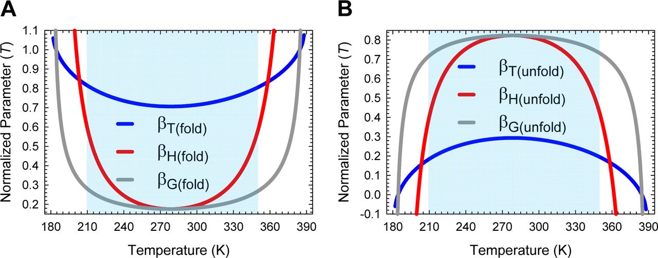
The position of the TSE relative to the ground states depends on the choice of the RC and changes in a complex manner with temperature. (A) For 210 K∽ < T < ∽350 K (shaded region), the position of the TSE relative to the DSE is the most advanced along the solvent RC as compared to the heat capacity and entropic RCs; and for T ≠ TS, is the most advanced along the heat capacity RC as compared to the entropic RC (B) In contrast, for 210 K∽ < T < ∽350 K and T ≠ TS, the position of the TSE relative to the NSE is the most advanced along the entropic RC as compared to the heat capacity RC, and is the least advanced along the SASA-RC.
Temperature-dependence of Φ-values
Φ-value analysis is a variation of the Brønsted procedure introduced by Fersht and coworkers which when properly implemented claims to provide a near-atomic-level description of the transiently populated reaction-states in protein folding.79,80 In this procedure, the primary sequence of the target protein is modified using protein engineering, and the effect of these perturbations are quantified through a parameter Φ (0 ≤ Φ ≤ 1) which by definition is the ratio of mutation-induced change in the Gibbs activation energy of folding/unfolding to the corresponding change in equilibrium stability. According to the canonical formulation, when ΦF(T) = 0 (Φ-value for folding), it implies that the energetics of the TSE is perturbed to the same extent as that of the DSE upon mutation, and hence inferred that the said reaction-states are structurally identical with respect to the site of mutation. In contrast, when ΦF(T) = 1, it implies that the energetics of the TSE is perturbed to the same extent as that of the NSE, and hence inferred that the structure at the site of mutation is identical in both the TSE and the NSE. Partial Φ-values are difficult to interpret and are thought to be due to partially developed interactions in the TSE, or multiple routes to the TSE. Thus, while Φ per se is the slope a two-point Brønsted plot, the conversion of this value to relative-structure is based on the Hammond postulate and the canonical range: The Hammond postulate provides the licence to infer structure from energetics, and the canonical scale enables one to infer how similar or dissimilar the TSE is to either the DSE or the NSE. Assuming that the prefactor is identical for the wild type and the mutant proteins, we may write for the partial folding (D ⇌ [TS]) and unfolding (N ⇌ [TS]) reactions

 where the subscripts “wt” and “mut” denote the reference or the wild type, and the structurally perturbed protein, respectively, and ΦU(T) is the Φ-value for unfolding. Inspection of Eqs. (42) and (43) shows that for a two-state system, ΦF(T) + ΦU(T) = 1. Now, although the primary sequence is intact in thermal denaturation experiments, we can readily calculate the temperature-dependence of Φ values for folding and unfolding using the protein at one unique temperature as the internal reference or the wild type, and protein at all the rest of the temperatures as the mutants. Thus, if the protein at TS is defined as the internal reference or the wild type, Eqs. (42) and (43) become


Similarly, if the protein at Tm is defined as the internal reference or the wild type, Eqs. (42) and (43) become

 Where x = ΔGTS-D(Tm) = ΔGTS-N(Tm) and y = ΔGN-D(T) ≡ −ΔGD-N(T) (the denominator reduces to a single quantity since ΔGD-N(Tm) ≡ −ΔGN-D(Tm) = 0). The parameters ΦF(internal)(T) and ΦU(internal)(T) (which are obviously undefined for the reference temperatures) when interpreted according to the canonical Φ-value framework (i.e., the notion that 0 ≤ Φ ≤ 1) are a measure of the global similarity or dissimilarity of the structure of the TSE to either the DSE or the NSE. Thus, if ΦF(internal)(T) = 0, it implies that the energetics of the TSE is perturbed to the same extent as that of the DSE upon a perturbation in temperature, and hence inferred that the global structure of the TSE is identical to that of the DSE. Conversely, if ΦF(internal)(T) = 1, it implies that the energetics of the TSE is perturbed to the same extent as the NSE upon a perturbation in temperature, and hence inferred that the global structure of the TSE is identical to that of the NSE.
Inspection of Figures 21 and Figure 21−figure supplements 1, 2, 3 and 4 immediately demonstrates that: (i) irrespective of which temperature is defined as the internal reference (i.e., the wild type), ΦF(internal)(T) must be a minimum and ΦU(internal)(T) must be a maximum at TS (see Appendix); (ii) the magnitude of ΦF(internal)(T) is always the least, and the magnitude of ΦU(internal)(T) is always the greatest when the protein at TS is defined as the reference or the wild type protein, and any deviation in the definition of the reference temperature from TS must lead to a uniform increase in ΦF(internal)(T) and a uniform decrease in ΦU(internal)(T) for all temperatures; (iii) although the algebraic sum of ΦF(internal)(T) and ΦU(internal)(T) is unity for all temperatures, the notion that they must independently be restricted to 0 ≤ Φ ≤ 1 is flawed; and (iv) although both Leffler βG(T) and Fersht Φ values are derived from changes in Gibbs activation energies for folding and unfolding relative to changes in equilibrium stability upon a perturbation in temperature, their response is not the same since the equations that govern their behaviour are not the same. While the magnitude of the Leffler βG(T) is independent of the reference owing to it being the ratio of the derivatives of the change in Gibbs energies with respect to temperature, the magnitude of Φ(internal)(T) is dependent on the definition of the reference state. For example, if the protein at TS is defined as the wild type, then βG(fold)(T) ≈ ΦF(internal)(T) and βG(unfold)(T) ≈ ΦU(internal)(T) around the temperature of maximum stability; but as the temperature deviates from TS, βG(fold)(T) increases far more steeply than ΦF(internal)(T), and βG(unfold)(T) decreases far more steeply than ΦU(internal)(T) such that for T ≠ TS we have βG(fold)(T) > ΦF(internal)(T) and βG(unfold)(T) < ΦU(internal)(T) (Figure 21−figure supplement 3). In contrast, if the protein at Tm is defined as the wild type, then we have: (i) βG(fold)(T) < ΦF(internal)(T) for Tc < T < Tm and βG(fold)(T) > ΦF(internal)(T) for T < Tc and T > Tm; and (ii) βG(unfold)(T) > ΦU(internal)(T) for Tc < T < Tm and βG(unfold)(T) < ΦU(internal)(T) for T < Tc and T > Tm(Figure 21−figure supplement 4). The point we are trying to make is that a comparison of the position of the TSE along Leffler βG(T) and Φ(internal)(T) RCs is not straightforward since both βG(T) and Φ(internal)(T) are temperature-dependent, and importantly respond differently to temperature-perturbation; and even if we restrict the comparison to one particular temperature, the answer we get is still subjective since the magnitude of Φ(internal)(T) is dependent on how we define the wild type.92

(A) ΦF(internal)(T) calculated using the protein at TS as the wild type must always be lower than ΦF(internal)(T) calculated using protein at T ≠ TS as the wild type. (B) ΦU(internal)(T) calculated using the protein at TS as the wild type must always be greater than ΦU(internal)(T) calculated using protein at T ≠ TS as the wild type. For the blue curves we have ΔG(wt) ≡ ΔG(TS), and for the red curves, we have ΔG(wt) ≡ ΔG(Tm). This notation applies to both equilibrium and activation energies. The blue curves are undefined (0/0) at TS, and the red curves are undefined at Tc and Tm. Note that the mathematical stipulation that ΦF(internal)(T) + ΦU(internal)(T) = 1 for a two-state system is satisfied for both the blue and the red curves for all temperatures.
Although the mathematical formalism for why the extrema of ΦF(internal)(T) (which is a minimum) and ΦU(internal)(T) (which is a maximum) must always occur precisely at TS has been shown in the appendix, it is instructive to examine the same graphically. Inspection of Figure 21−figure supplements 5, 6 and 7 demonstrates that this is a consequence of ΔGTS-D(T) and ΔGN-D(T) being a minimum, and ΔGTS-N(T) and ΔGD-N(T) being a maximum at TS. Subtracting the reference Gibbs energies from the numerator and the denominator (Eq. (44)) has the effect of lowering the ΔGTS-D(T) curve and raising the ΔGN-D(T), such that the value of the said curves are zero at the reference temperature, but the shapes of the curves are not altered in any way (Figure 21−figure supplement 5). On the other hand, for ΔGTS-N(T) and ΔGD-N(T) curves (Eq. (45)), apart from the value of the curves becoming zero at the reference, it causes them to flip vertically (Figure 21−figure supplement 6). Consequently, if we divide the transformed Gibbs activation energies by the transformed equilibrium Gibbs energies, we end up with ΦF(internal)(T) and ΦU(internal)(T) which are a minimum and a maximum, respectively, at TS (Figure 21−figure supplement 7).
Now that the process that leads to the temperature-dependence of Φ has been addressed, the question is “Can we infer the structure of the TSE as being similar to either the DSE or the NSE from these data?” The answer is “no” for several reasons. First, as argued earlier, the Hammond postulate cannot be valid for protein folding; and because the structural interpretation of Φ values is based on the Hammond postulate, it too must be deemed fallacious. Second, even if we accept the premise that Hammond postulate is applicable to protein folding, the inference that the global structure of the TSE as being denatured-like for ΦF(internal)(T) = 0, and native-like for ΦF(internal)(T) = 1 is flawed since Φ values need not necessarily be restricted to 0 ≤ Φ ≤ 1 (Figure 21−figure supplement 2). Third, even if we summarily exclude those wild types that lead to anomalous Φ values as being unsuitable for Φ analysis, we still have a problem since even within the restricted set of wild types that yield 0 ≤ Φ ≤ 1, their magnitude depends on the definition of the wild type; consequently, for the same temperature, the degree of structure in the TSE relative to that in the DSE appears to increase as the definition of the wild type deviates from TS (Figure 21−figure supplement 1). If we try to circumvent this interpretational problem by arguing that the “inference of the structure of the TSE” is always relative to the residual structure in the DSE, and that changing the definition of what constitutes the wild type will invariably affect Φ values, then we can’t really say much about the structure of the TSE without first solving the structure of the DSE. Fourth, even if through a judicious combination of various structural and biophysical methods (residual dipolar couplings, paramagnetic relaxation enhancement, small angle X-ray scattering, single molecule spectroscopy etc.), and computer simulation, we are able to determine the residual structure in the DSE,93-96 the structural interpretation of Φ values leads to physically unrealistic scenarios. For example, inspection of Figure 21A shows that around room temperature (298 K) ΦF(internal)(T) ≈ 0.18. A canonical interpretation of this number implies that the global structure of the TSE is very similar to that of the DSE. However, inspection of Figure 2−figure supplement 1A shows that the denatured conformer has buried ∽70% of the total SASA to reach the TSE (i.e., advanced by about 70% along the SASA-RC). Similarly, inspection of Figure 5A shows that ΔGTS-D(T) = 2.6 kcal.mol-1 at 298 K (note that this is not a small number that can be ignored since ΔGD-N(T) = 2.1 kcal.mol-1 at 298 K). Further, we have shown earlier in the section on the “Inapplicability of the Hammond postulate to protein folding,” that even when two reaction-states have identical SASA, Gibbs energies, enthalpies, and entropies, there need not necessarily have identical structure. Thus, the question is: How can we conclude with any measure of certainty that the global structure of the TSE is very similar to that of the DSE at 298 K when they have such a large difference in SASA, and a substantial difference in Gibbs energy? To illustrate why it is difficult to rationalize the theoretical basis of Φ analysis, it is instructive to directly examine the ratio of the Gibbs activation energies and the difference in Gibbs energy between the ground states (Figure 21−figure supplement 8). It is immediately apparent that the ratios are a complex function of temperature; and although we can readily provide an explanation for the particular features of these complex dependences, it is difficult to see how subtracting reference energies from the numerator and denominator of the ratios ΔGTS-D(T)/ΔGN-D(T) and ΔGTS-N(T)/ΔGD-N(T) allows us to divine the structure of the TSE to a near-atomic resolution. This is once again readily apparent from the complex non-linear relationship between equilibrium stability and the rate constants (Figure 21−figure supplement 9).

(A) ΦF(internal)(T) calculated by defining the protein at Tω as the wild type. (B) ΦU(internal)(T) calculated by defining the protein at Tω as the wild type. Although the mathematical stipulation that ΦF(internal)(T) + ΦU(internal)(T) = 1 for a two-state system is satisfied for all temperatures, Φ values for folding and unfolding are not restricted to the canonical range of 0 ≤ Φ ≤ 1 when the protein at Tω is defined as the reference or the wild type. Note that the curves are undefined at Tω.
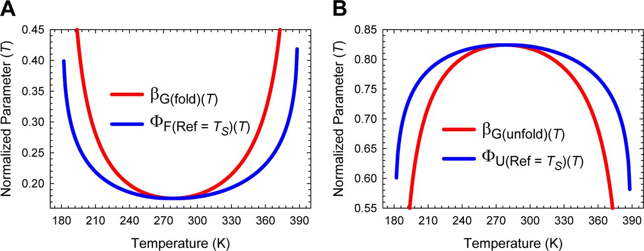
(A) βG(fold)(T) is almost identical to ΦF(internal)(T) around the temperature of maximum stability, but as the temperature deviates from TS, βG(fold)(T) increases far more steeply than ΦF(internal)(T), such that for T ≠TS we have βG(fold)(T) > ΦF(internal)(T). (B) βG(unfold)(T) is almost identical to ΦU(internal)(T) around the temperature of maximum stability, but as the temperature deviates from TS, βG(unfold)(T) decreases far more steeply than ΦU(internal)(T), such that for T ≠TS we have βG(unfold)(T) < ΦU(internal)(T).

(A) βG(fold)(T) < ΦF(internal)(T) for Tc < T < Tm and βG(fold)(T) > ΦF(internal)(T) for T < Tc and T > Tm. (B) βG(unfold)(T) > ΦU(internal)(T) for Tc < T < Tm and βG(unfold)(T) < ΦU(internal)(T) for T < Tc and T > Tm. Note that ΦF(internal)(T) and ΦU(internal)(T) are undefined for Tc and Tm (green pointers).

(A) The transformation ΔGTS-D(T) − ΔGTS-D(TS) (the numerator in Eq. (44)) lowers the ΔGTS-D(T) function such that the value of ΔΔGTS-D(T-TS) is zero at the reference temperature. (B) The transformation ΔGN-D(T) – ΔGN-D(TS) (the denominator in Eq. (44)) raises the ΔGN-D(T) function such that the value of ΔΔGN-D(T-TS) is zero at the reference temperature. The unmodified and the transformed curves are shown in black and red, respectively.

(A) The transformation ΔGTS-N(TS) − ΔGTS-N(T) (the numerator in Eq. (45)) flips the ΔGTS-N(T) function vertically and concomitantly shifts it along the ordinate such that the value of ΔΔGTS-N(TS-T) at the reference temperature is zero. (B) The transformation ΔGD-N(TS) – ΔGDN(T) (the denominator in Eq. (45)) flips the ΔGD-N(T) function vertically and concomitantly shifts it along the ordinate such that the value of ΔΔGD-N(TS-T) at the reference temperature is zero. The unmodified and the transformed curves are shown in black and red, respectively.

(A) Dividing ΔΔGTS-D(T-TS) by ΔΔGN-D(T-TS) generates ΦF(internal)(T) with its minimum at TS. (B) Dividing ΔΔGTS-N(TS-T) by ΔΔGD-N(TS-T) generates ΦU(internal)(T) with its maximum at TS. Note that the dimensions of the ordinate apply only to the red and the blue curves since Φ(internal)(T) is dimensionless.

(A) The ratio ΔGTS-D(T)/ΔGN-D(T) is negative for Tc < T < Tm and positive for T < Tc and T < Tm. (B) The ratio ΔGTS-N(T)/ΔGD-N(T) is positive for Tc < T < Tm and negative for T < Tc and T > Tm. The vertical asymptotes are a consequence of ΔGD-N(T) = −ΔGN-D(T) approaching zero as the temperature approaches Tc and Tm. Note that the ordinate is dimensionless, and that (ΔGTS-D(T)/ΔGN-D(T)) + (ΔGTS-N(T)/ΔGD-N(T)) = 1 for a two-state system.

(A) kf(T) vs the Gibbs energy of folding at equilibrium. The slope of this plot equals −kf(T) ΔHTS-D(T)/ΔSTS-D(T)/ΔSN-D(T)RT2. (B) ku(T) vs the Gibbs energy of unfolding at equilibrium. The Marcus-inverted-regimes which occur at very low and high temperatures are towards the extreme left. The slope of this plot is given by −ku(T) ΔHTS-D(T)/ΔSTS-D(T)/ΔSN-D(T)RT2. (C) Natural logarithm of kf(T) vs the Gibbs energy of folding at equilibrium (slope = -ΔHTS-D(T)/ΔSN-D(T)RT2). (D) Natural logarithm of ku(T) vs the Gibbs energy of unfolding at equilibrium (slope = -ΔHTS-D(T)/ΔSN-D(T)RT2). The abscissae for plots A and C, and plots B and D are identical. The colour-code is identical for all the four plots.

(A) Temperature-dependence of ΦF(internal)(T). (B) Temperature-dependence of ΦU(internal)(T). The red pointers indicate the extrema of the functions. The discontinuities in the curves which must occur at TS have been removed by mathematically manipulating Eqs. (42) and (45) (manipulated equations not shown). Nevertheless, ΦF(internal)(T) and ΦU(internal)(T) are undefined at TS (i.e., the curves have holes at TS which is not obvious). Note that the mathematical stipulation that ΦF(internal)(T) + ΦU(internal)(T) = 1 for a two-state system is satisfied for all temperatures.
To further illuminate the difficulty in rationalizing the Φ-value procedure, it is instructive to apply Eqs. (42) and (45) to treat enthalpies. Thus, for the partial folding (D ⇌ [TS]) and unfolding (N ⇌ [TS]) reactions we have

 Where the parameters ΦHF(internal)(T) and ΦHU(internal)(T) are the “enthalpic analogues” of ΦF(internal)(T) and ΦU(internal)(T), respectively (the subscript “H” indicates we are using enthalpy instead of Gibbs energy), when the protein at the temperature TS is defined as the wild type. Now, if we apply an analogous version of the canonical interpretation given by Fersht and coworkers, it implies that when ΦHF(internal)(T) = 0, the enthalpy of the TSE is perturbed to the same extent as that of the DSE upon a perturbation in temperature; and when ΦHF(internal)(T) = 1, it implies that the enthalpy of the TSE is perturbed to the same extent as that of the NSE. It is easy to see that just as ΦF(internal)(T) and ΦU(internal)(T) are the Fersht-analogues of the Leffler βG(fold)(T) and βG(unfold)(T), respectively (see entropic RC), the parameters ΦHF(internal)(T) and ΦHU(internal)(T) are similarly the Fersht-analogues of the Leffler βH(fold)(T) and βH(unfold)(T), respectively (see heat capacity RC).
Inspection of Figure 22 and its supplements immediately demonstrates that the same anomalies that prevent a straightforward structural interpretation of ΦF(internal)(T) and ΦU(internal)(T) are also emerge if we try to assign structure to their enthalpic analogues, ΦHF(internal)(T) and ΦHU(internal)(T). First, although the algebraic sum of ΦHF(internal)(T) and ΦHU(internal)(T) is unity for all temperatures, they need not independently be restricted to a canonical range of 0 ≤ Φ ≤ 1 (Figure 22). Second, the magnitude of ΦHF(internal)(T) and ΦHU(internal)(T) are dependent on the definition of the wild type (Figure 22−figure supplement 1). Third, changing the definition of the wild type has a dramatic effect on the relationship between the Leffler βH(T) and its analogue, the Fersht ΦH(internal)(T). Consequently, the question of whether Leffler βH(T) underestimates or overestimates structure is dependent on how we analyse the system (Figure 22−figure supplements 2 and 3). Fourth, just as the temperature-dependent position of the TSE relative to the ground states depends on the choice of the RC (Figure 20), we see that Φ(internal)(T) and its enthalpic analogue, ΦH(internal)(T), change at different rates upon a perturbation in temperature (Figure 22−figure supplement 4). The difficulty in rationalizing how subtracting reference values from the numerator and the denominator of Eqs. (42) and (49) can yield residue-level information is once again apparent from the complex dependence of the ratios ∂ ln kf(T)/∂ ln KN-D(T) = ΔHTS-D(T)/ΔHN-D(T) and ∂ ln ku(T)/∂ ln KD-N(T) = ΔHTS-N(T)/ΔHD-N(T) on temperature (Figure 22−figure supplement 5).

(A) A comparison of ΦHF(internal)(T) calculated using proteins at TS and Tm as the wild types. (B) A comparison of ΦHU(internal)(T) calculated using proteins at TS and Tm as the wild types. For the blue curves we have ΔH(wt) ≡ ΔH(TS), and for the red curves, we have ΔH(wt) ≡ ΔH(Tm). This notation applies to both equilibrium and activation enthalpies. The blue curves are undefined (0/0) at TS, and the red curves are undefined at Tc and Tm. This figure is the enthalpic equivalent of Figure 21−figure supplement 1.

(A) βH(fold)(T) is almost identical to ΦHF(internal)(T) around the temperature of maximum stability, but as the temperature deviates from TS, βH(fold)(T) increases far more steeply than ΦHF(internal)(T), such that for T ≠TS we have βH(fold)(T) > ΦHF(internal)(T). (B) βH(unfold)(T) is almost identical to ΦHU(internal)(T) around the temperature of maximum stability, but as the temperature deviates from TS, βH(unfold)(T) decreases far more steeply than ΦHU(internal)(T), such that for T ≠TS we have βH(unfold)(T) < ΦHU(internal)(T). Note that the parameters ΦHF(internal)(T) and ΦHU(internal)(T) are the Fersht-analogues of the Leffler βH(fold)(T) and βH(unfold)(T), respectively (see heat capacity RC). Consequently, this figure is analogous to a comparison of Leffler βG(fold)(T) and Fersht ΦF(internal)(T), and Leffler βG(unfold)(T) and Fersht ΦU(internal)(T) (see Figure 21−figure supplement 3).

Changing the definition of the wild type from TS (see previous figure) to Tm has a dramatic effect on the relationship between the Leffler-βH(T) and the Fersht-ΦH(internal)(T). (A) βH(fold)(T) < ΦHF(internal)(T) for ∽248 K < T < Tm, βH(fold)(T) > ΦHF(internal)(T) for T < ∽248 K and T > Tm, and identical when T = ∽248 K. (B) βH(unfold)(T) > ΦHU(internal)(T) for ∽248 K < T < Tm, βH(unfold)(T) < ΦHU(internal)(T) for T < ∽248 K and T > Tm, and identical when T = ∽248 K. Note that ΦHF(internal)(T) and ΦHU(internal)(T) are undefined at Tm and the discontinuity in the functions is apparent upon close inspection. This figure is the enthalpic equivalent of Figure 21−figure supplement 4.

(A) The normalized Gibbs parameter ΦF(internal)(T) is almost identical to the normalized enthalpic parameter ΦHF(internal)(T) around the temperature of maximum stability, but as the temperature deviates from TS, ΦHF(internal)(T) increases far more steeply than ΦF(internal)(T), such that for T ≠TS we have ΦHF(internal)(T) > ΦF(internal)(T). (B) The normalized Gibbs parameter ΦU(internal)(T) is almost identical to the normalized enthalpic parameter ΦHU(internal)(T) around the temperature of maximum stability, but as the temperature deviates from TS, ΦHU(internal)(T) decreases far more steeply than ΦU(internal)(T), such that for T ≠TS we have ΦHF(internal)(T) < ΦU(internal)(T). Since Φ(internal)(T) and ΦH(internal)(T) are the Fersht-analogues of Leffler βG(T) and βH(T), respectively, this figure is analogous to comparing the temperature-dependent position of the TSE along the entropic and heat capacity RCs (i.e., a comparison of the temperature-dependence of βG(T) and βH(T); see Figure 17).

(A) The ratio ΔHTS-D(T)/ΔHN-D(T) is positive for Tα ≤ T < TH and TH(TS-D) < T ≤ Tω, negative for TH < T < TH(TS-D) and zero at TH(TS-D). (B) The ratio ΔHTS-N(T)/ΔHD-N(T) is positive for TS(α) < T < TH(TS-N) and TH < T < TS(ω), negative for Tα ≤ T < TS(α), TH(TS-N) < T < TH, and TS(ω) < T ≤ Tω, and zero at TS(α), TH(TS-N), and TS(α). The vertical asymptotes are a consequence of ΔHD-N(T) = −ΔHN-D(T) approaching zero as T→TH. Note that the ordinate is dimensionless, and that (ΔHTS-D(T)/ΔHN-D(T))+(ΔHTS-N(T)/ΔHD-N(T))=1 for a two-state system.

(A) Temperature-dependence of ΦHF(internal)(T). (B) Temperature-dependence of ΦHU(internal)(T). Note that both these curves are undefined at TS. Although the algebraic sum of ΦHF(internal)(T) and ΦHU(internal)(T) is unity for all temperatures, they need not necessarily be are not restricted to a canonical range of 0 ≤ Φ ≤ 1. The parameters ΦHF(internal)(T) and ΦHU(internal)(T) are the “enthalpic analogues” of ΦF(internal)(T) and ΦU(internal)(T), respectively (the subscript “H” indicates we are using enthalpy instead of Gibbs energy). Consequently, this figure is the enthalpic equivalent of Figure 21.
Comparison of theoretical and experimental Φ-values obtained from structural perturbation across 31 two-state systems
Given that the framework of Φ-value analysis was primarily developed to be used in conjunction with structural rather than temperature perturbation, and despite its anomalies has been used extensively for more than twenty years to divine the structures of the TSEs of not just globular but also membrane proteins, it is imperative to demonstrate that the notion that the structure of the TSE cannot be inferred from Φ-values is also valid for structural perturbation.97-101 Although a detailed reappraisal is beyond the scope of this article and will be presented elsewhere, because we have questioned the validity of Φ analysis, one is compelled to provide some justification in this article.
Consider the wild type of a hypothetical two-state folder whose equilibrium stability and the mean length of the RC at constant temperature, pressure and solvent conditions are given by ΔGD-N(T) = 6 kcal.mol-1 and mD-N = 2 kcal.mol-1.M-1, respectively. Although not necessarily true and addressed elsewhere, to limit the number of hypothetical scenarios to a manageable number, we will assume that the force constants of the DSE and the NSE-parabolas of the wild type and all its mutants are given by α = 1 M2.mol.kcal-1 and ω = 30 M2.mol.kcal-1. The effect of single point mutations on the wild type may be classified into a total of five unique scenarios (Figure 23A).
Case I (Quadrant x2): The introduced mutation causes a concomitant decrease in both the stability and the mean length of the RC (i.e., ΔGD-N(T)(wt) > ΔGD-N(T)(mut) and mD-N(wt) > mD-N(mut)). This is equivalent to the introduced mutation causing the separation between the vertices of the DSE and the NSE-parabolas along the abscissa and ordinate to decrease (Figure 23−figure supplement 1A).

The parabolas corresponding to the DSE and NSE of the wild type are shown in black in all the four plots. The mutant DSE-parabolas are shown in blue and red while the mutant NSEparabolas are shown in magenta. (A) The introduced mutation causes a concomitant decrease in ΔGD-N(T) and the mean-length of the RC. (B) The introduced mutation causes a decrease in ΔGD-N(T) but an increase in the mean-length of the RC. (C) The introduced mutation stabilizes the mutant but causes a concomitant decrease in the mean-length of the RC. (D) The introduced mutation stabilizes the protein but concomitantly causes an increase in the mean-length of the RC. The curvatures of all the DSE-parabolas (α = 1 M2.mol.kcal-1) and all the NSE-parabolas (ɷ = 30 M2.mol.kcal-1) are identical.
Case II (Quadrant y1): The introduced mutation causes a decrease in stability but concomitantly causes an increase in the mean length of the RC (i.e., ΔGD-N(T)(wt) > ΔGD-N(T)(mut) and mD-N(wt) < mD-N(mut)). This is equivalent to the mutation causing a decrease in the separation between the vertices of the DSE and the NSE-parabolas along the ordinate, but an increase along the abscissa (Figure 23−figure supplement 1B).
Case III (Quadrant x1): The introduced mutation leads to an increase in stability but concomitantly causes a decrease in the mean length of the RC (i.e., ΔGD-N(T)(wt) < ΔGD-N(T)(mut) and mD-N(wt) > mD-N(mut)). This is equivalent to the mutation causing an increase in the separation between the vertices of the DSE and the NSE-parabolas along the ordinate, but a decrease along the abscissa (Figure 23−figure supplement 1C).
Case IV (Quadrant y2): The introduced mutation leads to a concomitant increase in both the stability and the mean length of the RC (i.e., ΔGD-N(T)(wt) < ΔGD-N(T)(mut) and mD-N(wt) < mD-N(mut)). This is equivalent to the mutation causing an increase in the separation between the vertices of the DSE and the NSE-parabolas along the ordinate and the abscissa (Figure 23−figure supplement 1D).
Case V: The introduced mutation leads to a change in stability but has no effect on the mean length of the RC (mD-N(wt) = mD-N(mut)). This is equivalent to the mutation causing an increase or a decrease in the separation between the vertices of the DSE and the NSE-parabolas along the ordinate, but the separation along the abscissa is invariant (Figure 23−figure supplement 2).

The wild type DSE and NSE-parabolas are shown in black, the destabilized mutants are shown in red and blue, and the stabilized mutants are shown in green and magenta. As the protein is increasingly destabilized the curve-crossing along the RC shifts closer to the vertex of the NSE-parabola, and can be due to a stabilized DSE or a destabilized NSE, or both. Conversely, as the protein is increasingly stabilized, the curve-crossing along the RC shifts away from the vertex of NSE-parabola and this can be due to a destabilized DSE or a stabilized NSE, or both. The force constant for the DSE-parabola is α = 1 M2.mol.kcal-1. The curvatures of all the NSE-parabolas are identical (ɷ = 30 M2.mol.kcal-1).

(A) Theoretical limits of ΦF(T) values according to parabolic approximation where all the 1463 theoretical mutants have the following common parameters: α = 1 M2.mol.kcal-1 (DSE-parabola); ω = 30 M2.mol.kcal-1 (NSE-parabola). The wild type was arbitrarily chosen to be the one with parameters ΔGD-N(T)= 6 kcal.mol-1 and mD-N = 2 kcal.mol-1.M-1. The legend indicates the variation in mD-N values in kcal.mol-1.M-1. The quadrants labelled x1 and x2 are for mutants whose mD-N < mD-N(wt) (i.e., a contraction of the RC) and the quadrants labelled y1 and y2 are for those mutants whose mD-N > mD-N(wt) (i.e., an expansion of the RC). Close inspection shows that for those mutants whose stabilities have changed but not their mD-N values, the ΦF(T) values are positive but very close to zero (shown in cyan). Theoretical ΦF values corresponding to ΔΔGD-N(wt-mut)(T) = 0.0 ± 0.4 kcal.mol-1 have been excluded for clarity. This corresponds to about 6.7% error on the wild type ΔGD-N(wt)(T). (B) An overlay of theoretical ΦF(T) and experimental ΦF(T) values in water for 1035 mutants from 31 two-state systems. Data used to calculate the experimental ΦF(T) values were taken from published literature (detailed information is given elsewhere). The vertical asymptotes are a consequence of ΔΔGD-N(wt-mut)(T) approaching zero.
In summary, what we done is taken a pair of intersecting parabolas of differing curvature (ω > α), and systematically varied the separation between their vertices along the abscissa (mD-N) and ordinate (ΔGD-N(T)) without changing the curvature of the parabolas. Once this is done, we can calculate a priori the position of the curve-crossings relative to the vertex of the DSE-parabola along the abscissa (i.e., mTS-D(T); Eq. (1)) and ordinate (i.e., ΔGTS-D(T); Eq. (3)). Once the ΔGTS-D(T) values for all combinations of ΔGD-N(T) and mD-N are obtained (each combination is equivalent to a point mutation), ΦF(T) values can be readily calculated using Eq. (50) by arbitrarily choosing one particular combination of ΔGD-N(T) (= 6 kcal.mol-1) and mD-N (= 2 kcal.mol-1.M-1) as the wild type.

Figure 23A which has been generated by plotting the theoretical ΦF(T) values as a function of ΔΔGD-N(wt-mut)(T) leads to two important conclusions: (i) ΦF(T) values are not restricted to 0 ≤ Φ ≤ 1, and that the perceived unusualness of anomalous or non-classical Φ values is a consequence of flawed canonical limits; and (ii) the magnitude of ΦF(T) values decrease as the difference in stability between the wild type and the mutant proteins increase, and at once debunks the idea that one must use an arbitrary ΔΔGD-N(wt-mut)(T) cut-off (± 0.6 kcal.mol-1 according to the Fersht lab, and ± 1.7 kcal.mol-1 according to Sanchez and Kiefhaber) for ΦF(T) values to be interpretable.98,102 While it is true that Φ values would be error prone when |ΔΔGD-N(wt-mut)(T)| is less than the error with which one can determine ΔGD-N(T) of both the wild type and the mutant proteins (typically about ± 5-10% of ΔGD-N(T)),103 the increase in the magnitude of ΦF(T) values when ΔΔGD-N(wt-mut)(T) approaches zero (the vertical asymptotes) is a mathematical certainty and not because of error as is commonly argued. Nevertheless, because these conclusions are based on the results of a model that is purely hypothetical, they would naturally be meaningless without experimental validation. Thus, as a test of the hypothesis, experimental ΦF(T) values in water were calculated according to Eq. (51) using published kinetic data of a total of 1064 proteins (1035 mutants + 29 wild types) from 31 two-state systems (details of the systems analysed will be provided elsewhere).

The remarkable agreement between theoretical prediction and experimental ΦF(T) values is immediately apparent from an overlay of the said datasets (Figure 23B), and serves as arguably one of the most rigorous tests of the hypothesis for the following reasons: (1) The space enclosed by the curves in Figure 23A is complex and restricted. Therefore, if the experimental ΦF(T) values fall within this restricted theoretical space it would be highly unlikely for it to be purely due to some dramatic coincidence. (2) The sample size of experimental dataset is sufficiently large (1035 mutations), and the two-state systems investigated include α, β, and α/β proteins (note that α and β refer to secondary structure in this context and not to the force constant of the DSE or the Tanford beta value, respectively), with size ranging from 37 to 107 residues. (3) The published kinetic data used to calculate experimental ΦF(T) values were acquired by various labs under varying solvent conditions (buffers, co-solvents and pH; denaturant is either guanidine hydrochloride or urea) and temperature (as low as 278 K to as high as 301.16 K), over a period of about two decades using a variety of experimental methods, including infrared laser-induced and electrical discharge temperature-jump relaxation measurements, stopped flow and manual mixing experiments, and lineshape analysis of exchange-broadened NMR resonances. These results, including those on the temperature-dependence of ΦF(T) values lead to an important conclusion: Because the canonical scale itself has no basis, Φ-value-based interpretation of the structure of the transiently populated protein reaction-states is dubious.
Concluding Remarks
Although the temperature-dependent behaviour of FBP28 WW was analysed in great detail using the theory developed in the Papers I and II, and novel conclusions have been drawn, this is by no means sufficient since we have barely addressed the physical chemistry underlying the effect of temperature on the Gibbs energies, the enthalpies, the entropies, and the heat capacities of activation for folding and unfolding. These aspects will be dealt with in the accompanying articles. Further, there is a good reason why we have given little importance to the actual values of the reference temperatures and instead focussed on what they actually mean and how they relate to each other. Although the remarks in Table 1 are valid for all reference temperatures, except for the values of the equilibrium reference temperatures (Tc, TH, TS, and Tm), the values for the rest of them can change depending on the values of the force constants. However, what will not change is the inter-relationship between them. The nature of this limitation will be addressed when the mechanism of action of denaturants is investigated.
Methods
The temperature-dependence of ΔGD-N(T) of FBP28 WW wild type (Figure 1) was simulated according to Eq. (A1) using Tm = 337.2 K, ΔHD-N(Tm) = 26.9 kcal.mol-1 and ΔCpD-N = 417 cal.mol-1.K-1 (Table 1 in Petrovich et al., 2006).4 The values of k0 = 2180965 s-1, α = 7.594 M2.mol.kcal-1, ω = 85.595 M2.mol.kcal-1, and mD-N = 0.82 kcal.mol-1.M-1 were extracted from the chevron of FBP28 WW (acquired at 283.16 K in 20 mM 3-[morpholino] propanesulfonic acid, ionic strength adjusted to150 mM with Na2SO4, pH 6.5) by fitting it to a modified chevron-equation using non-linear regression as described in Paper-I. The data required to simulate the chevron (kf(H2O)(T), ku(H2O)(T), mTS-D(T) and mTS-N(T)) were taken from Table 4 in Petrovich et al., 2006.4 Once the parameters ΔHD-N(Tm), Tm, ΔCpD-N, mD-N, the force constants α and ω, and k0 are known, the left-hand side of all the equations in this article may be readily calculated for any temperature. Note that the spring constants, k0, mD-N, and ΔCpD-N are temperature-invariant.
Competing Financial Interests
The author declares no competing financial interests.
Appendix
The temperature-dependence of ΔGD-N(T), ΔHD-N(T), and ΔSD-N(T) functions
The temperature-dependence of the change in Gibbs energy, enthalpy and entropy of two-state systems upon unfolding at equilibrium are given by6


Where ΔHD-N(T), ΔHD-N(Tm) and ΔSD-N(T), ΔSD-N(Tm) denote the equilibrium enthalpies and entropies of unfolding, respectively, at any given temperature, and at the midpoint of thermal denaturation (Tm), respectively, for a given two-state folder under defined solvent conditions. The temperature-invariant and the temperature-dependent difference in heat capacity between the DSE and NSE are denoted by ΔCpD-N and ΔCpD-N(T), respectively.
The first derivatives of mTS-D(T), mTS-N(T), βT(fold)(T) and βT(unfold)(T) with respect to temperature
The first derivative of mTS-D(T) is given by

Because βT(fold)(T) = mTS-D(T)/mD-N, we also have

Since ∂mTS-D(T)/∂T and ∂βT(fold)(T)/∂T are physically undefined for φ < 0, their algebraic sign at any given temperature is determined by the ln(T/TS) term. This leads to three scenarios: (i) for T < TS we have ∂mTS-D(T)/∂T > 0 and ∂βT(fold)(T)/∂T > 0; and (iii) for T = TS we have ∂mTS-D(T)/∂T = 0 and ∂βT(fold)(T)/∂T = 0.
Because mTS-N(T) = (mD-N − mTS-D(T)) for a two-state system, and βT(unfold)(T) = mTS-N(T)/mD-N, we have


Eqs. (A6) and (A7) once again lead to three scenarios: (i) for T < TS we have ∂mTS-N(T)/∂T > 0 and ∂βT(unfold)(T)/∂T > 0; (ii) for T > TS we have ∂mTS-N(T)/∂T < 0 and ∂βT(unfold)(T)/∂T > 0; and (iii) for T = TS we have ∂mTS-N(T)/∂T = 0 and ∂βT(unfold)(T)/∂T = 0.
The second derivatives of mTS-D(T) and mTS-N(T) with respect to temperature
Differentiating Eq. (A4) with respect to temperature gives

Simplifying Eq. (A8) yields

Similarly, we may show that

Expression for the temperature-dependence of the observed rate constant
The observed rate constant kobs(T) for a two-state system is the sum of kf(T) and ku(T).104 Therefore, we can write


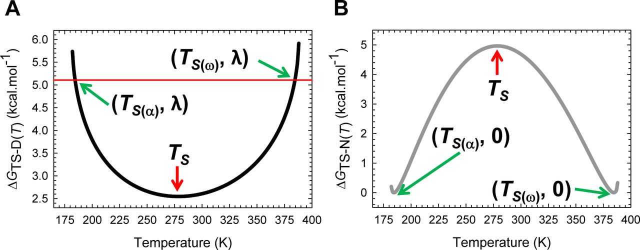
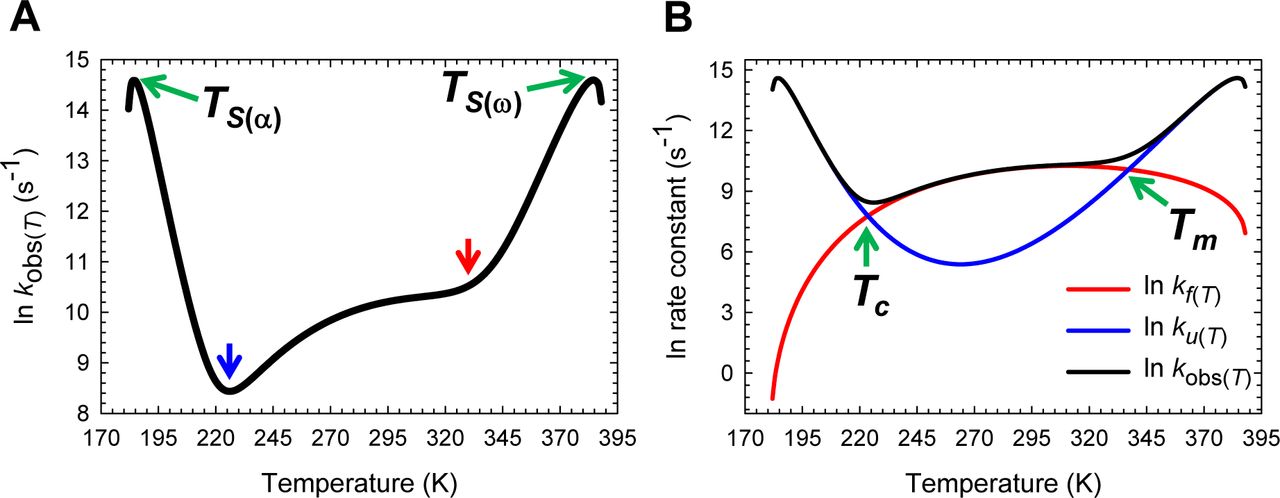
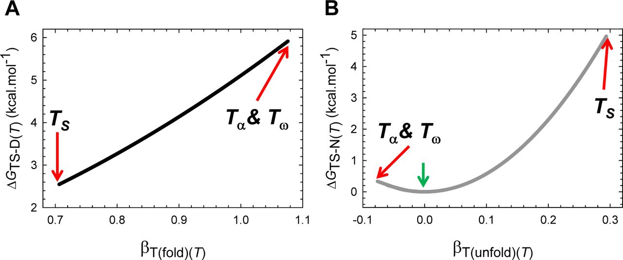
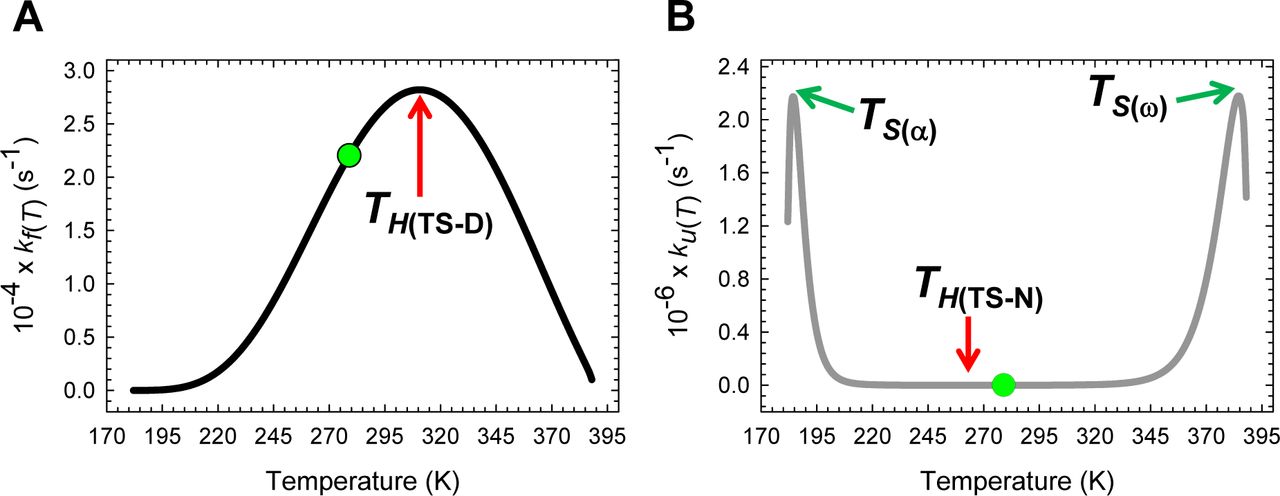
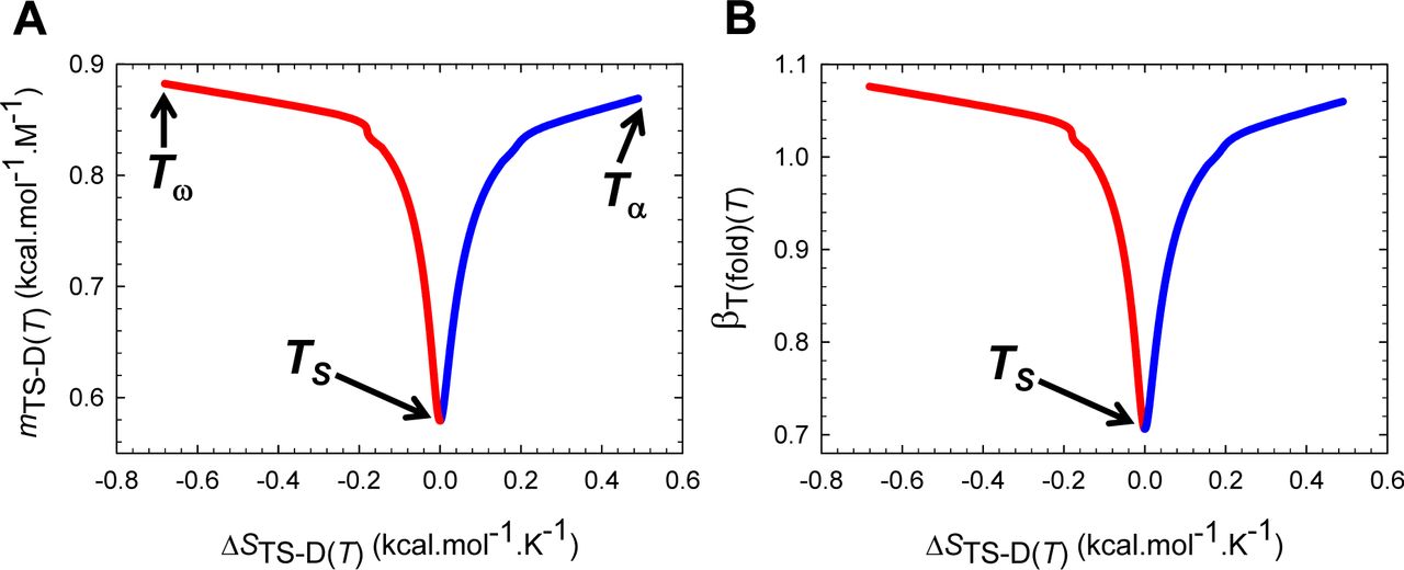
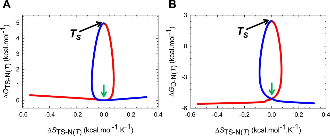
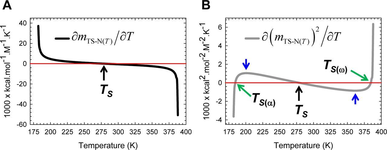
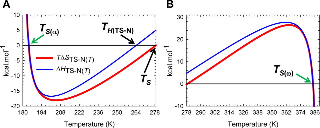
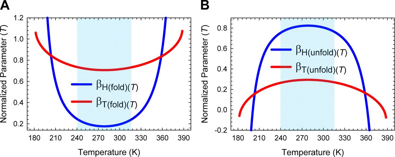
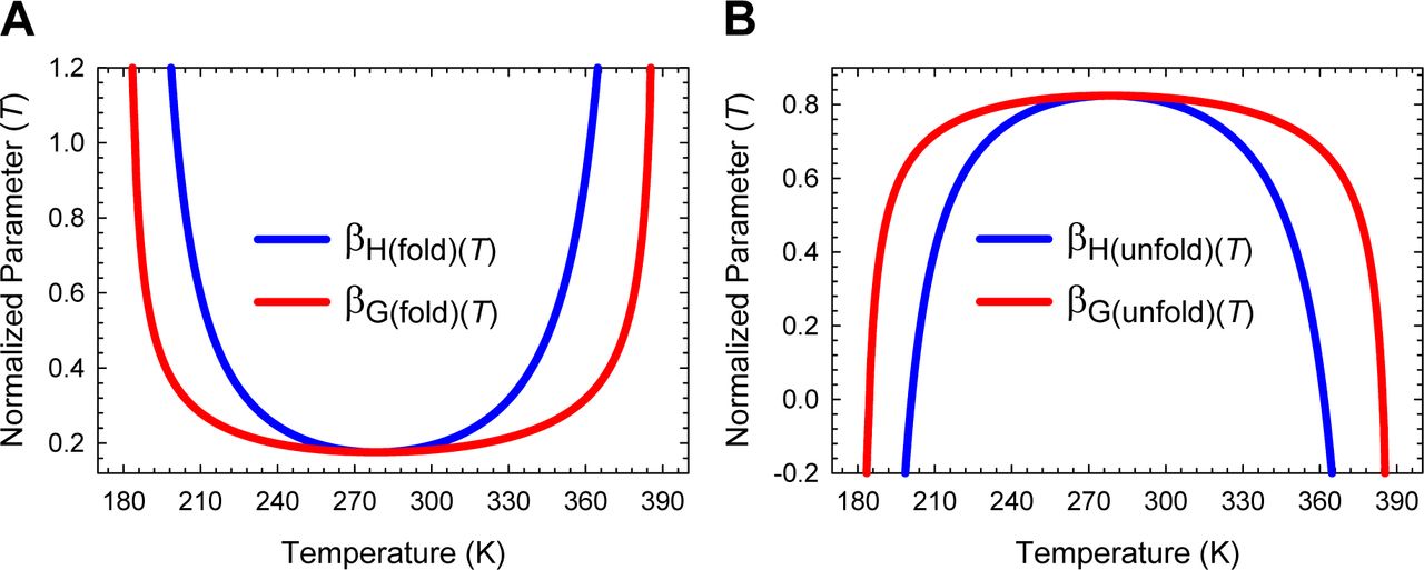
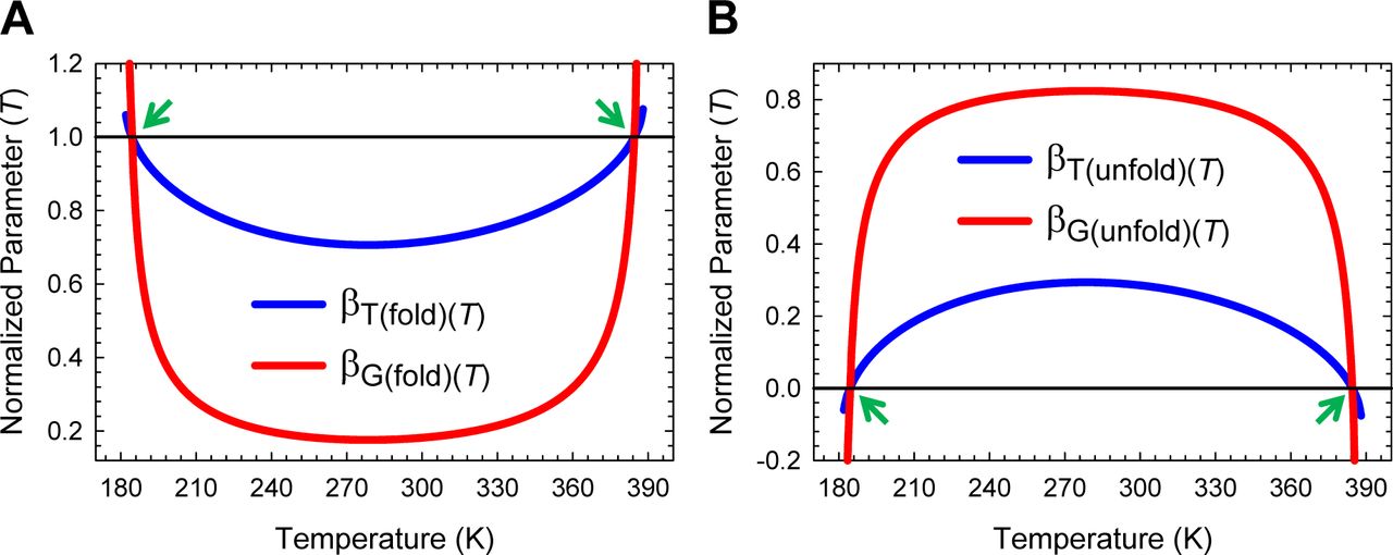
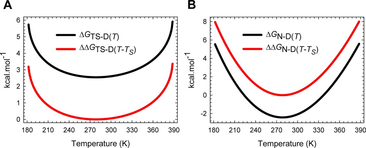
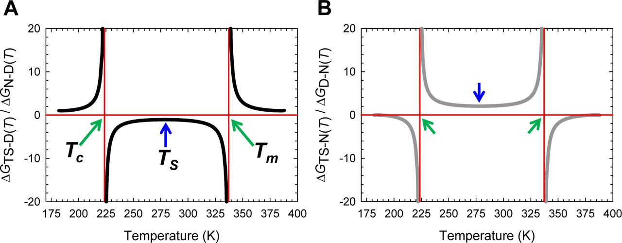
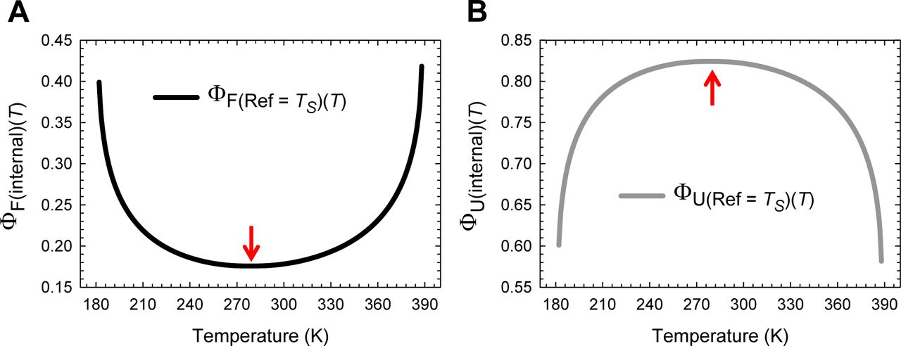
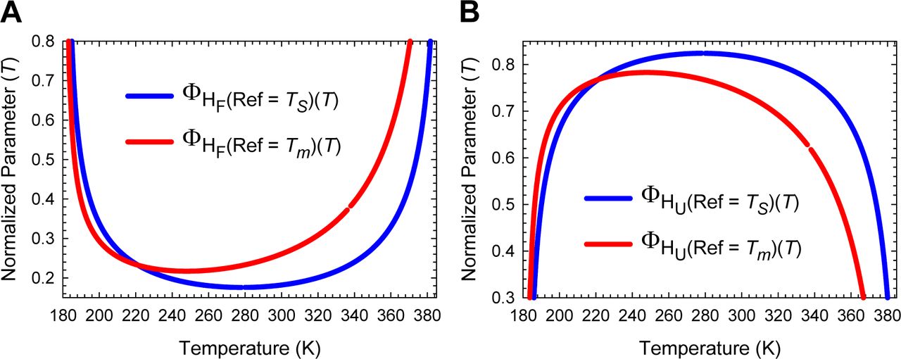
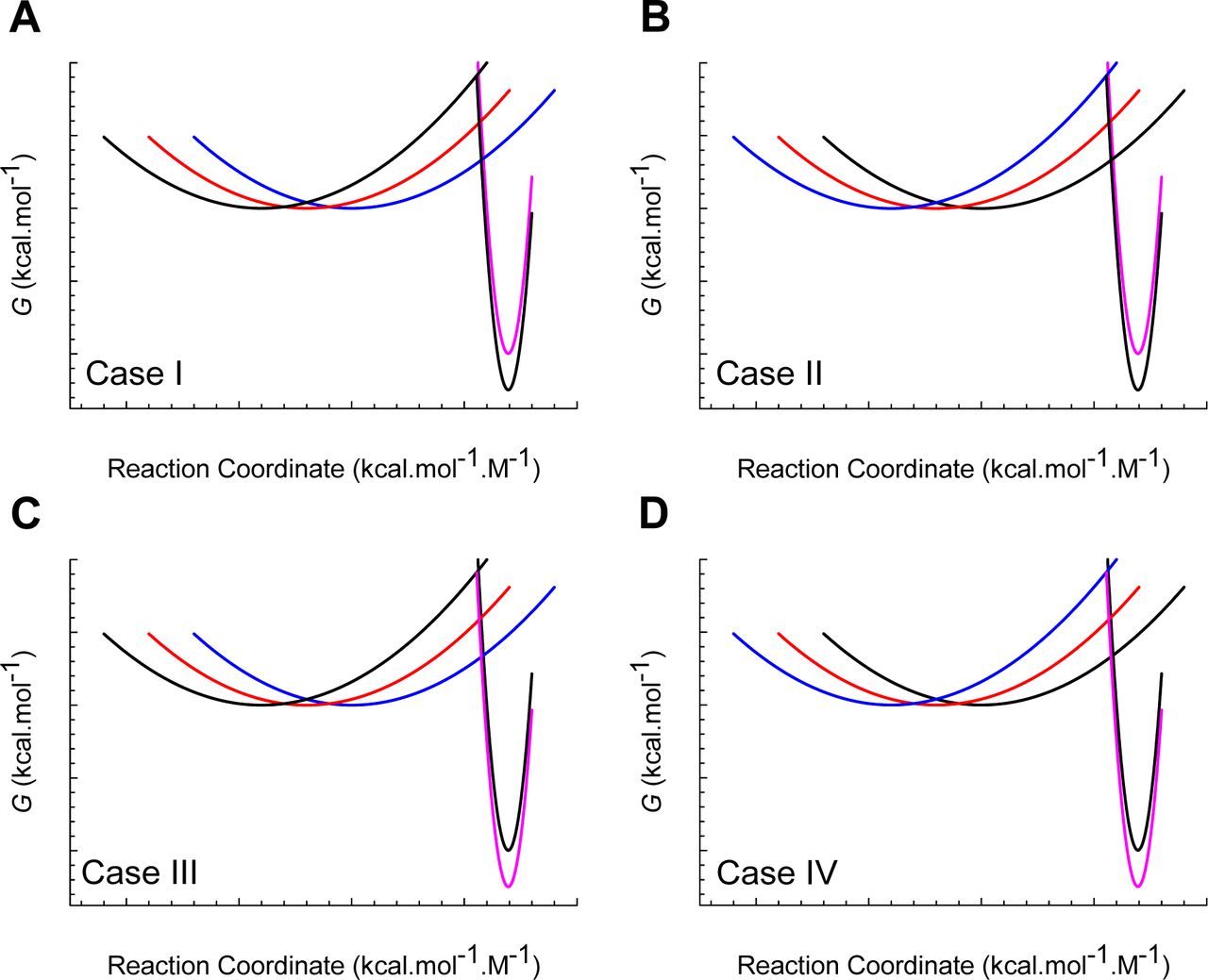
Expressions to demonstrate why the extrema of ΦF(internal)(T) and ΦU(internal)(T) must occur at TS
Differentiating Eq. (44) with respect to temperature gives

 where the protein at the temperature TRef is by definition the wild type protein. Because ΔSN-D(T) and ΔSTS-D(T) are both zero at TS, irrespective of TRef, the derivative of ΦF(internal)(T) will be zero at TS. Similarly, we can show by differentiating Eq. (45) that

Once again, since ΔSD-N(T) and ΔSTS-N(T) are both zero at TS, irrespective of TRef, the derivative of ΦU(internal)(T) will be zero at TS.
Footnotes
Vinkensteynstraat 128, 2562 TV, Den Haag, Netherlands, robert.sade{at}gmail.com
REFERENCES


