

Abstract
Convergent evolution occurs when multiple species/subpopulations adapt to similar environments via similar phenotypes. We investigate here the molecular basis of convergent adaptation in maize to highland climates in Mexico and South America using genome-wide SNP data. Taking advantage of archaeological data on the arrival of maize to the highlands, we infer demographic models for both populations, identifying evidence of a strong bottleneck and rapid expansion in South America. We use these models to then identify loci showing an excess of differentiation as a means of identifying putative targets of natural selection, and compare our results to expectations from recently developed theory on convergent adaptation. Consistent with predictions across a wide array of parameter space, we see limited evidence for convergent evolution at the nucleotide level in spite of strong similarities in overall phenotypes. Instead, we show that selection appears to have predominantly acted on standing genetic variation, and that introgression from wild teosinte populations appears to have played a role in highland adaptation in Mexican maize.
Introduction
Convergent evolution occurs when multiple species or populations exhibit similar phenotypic adaptations to comparable environmental challenges (Wood et al. 2005; Arendt and Reznick 2008; Elmer and Meyer 2011). Evolutionary genetic analysis of a wide range of species has provided evidence for multiple pathways of convergent evolution. One such route occurs when identical mutations arise independently and fix via natural selection in multiple populations. In humans, for example, malaria resistance due to mutations from Glu to Val at the sixth codon of the β-globin gene has arisen independently on multiple unique haplotypes (Currat et al. 2002; Kwiatkowski 2005). Convergent evolution can also be achieved when different mutations arise within the same locus yet produce similar phenotypic effects. Grain fragrance in rice appears to have evolved along these lines, as populations across East Asia have similar fragrances resulting from at least eight distinct loss-of-function alleles in the BADH2 gene (Kovach et al. 2009). Finally, convergent evolution may arise from natural selection acting on standing genetic variation in an ancestral population. In the three-spined stickleback, natural selection has repeatedly acted to reduce armor plating in independent colonizations of freshwater environments. Adaptation in these populations occurred both from new mutations as well as standing variation at the Eda locus in marine populations (Colosimo et al. 2005).
Not all convergent phenotypic evolution is the result of convergent evolution at the molecular level, however. Recent studies of adaptation to high elevation in humans, for example, reveal that the genes involved in highland adaptation are largely distinct among Tibetan, Andean and Ethiopian populations (Bigham et al. 2010; Scheinfeldt et al. 2012; Alkorta-Aranburu et al. 2012). While observations of independent origin may be due to a complex genetic architecture or standing genetic variation, introgression from related populations may also play a role. In Tibetan populations, the adaptive allele at the EPAS1 locus appears to have arisen via introgression from Denisovans, a related hominid group (Huerta-Sánchez et al. 2014). Overall, we still know relatively little about how convergent phenotypic evolution is driven by common genetic changes or the relative frequencies of these different routes of convergent evolution.
The adaptation of maize to high elevation environments (Zea mays ssp. mays) provides an excellent opportunity to investigate the molecular basis of convergent evolution. Maize was domesticated from the wild teosinte Zea mays ssp. parviglumis (hereafter parviglumis) in the lowlands of southwest Mexico ~9,000 years before present (BP) (Matsuoka et al. 2002; Piperno et al. 2009; van Heerwaarden et al. 2011). After domestication, maize spread rapidly across the Americas, reaching the lowlands of South America and the high elevations of the Mexican Central Plateau by ∼ 6,000 BP (Piperno 2006), and the Andean highlands by ∼ 4,000 BP (Perry et al. 2006; Grobman et al. 2012). The transition from lowland to highland habitats spanned similar environmental gradients in Mesoamerica and S. America (Figure S1) and presented a host of novel challenges that often accompany highland adaptation including reduced temperature, increased ultraviolet radiation, and reduced partial pressure of atmospheric gases (Körner 2007).
Common garden experiments in Mexico reveal that highland maize has successfully adapted to high elevation conditions (Mercer et al. 2008), and phenotypic comparisons between Mesoamerican and S. American populations are suggestive of convergent evolution. Maize landraces (open-pollinated traditional varieties) from both populations share a number of phenotypes not found in lowland populations, including dense macrohairs and stem pigmentation (Wilkes 1977; Wellhausen et al. 1957) and differences in tassel branch and ear husk number (Brewbaker 2014), and biochemical response to UV radiation (Casati and Walbot 2005). In spite of these shared phenotypes, genetic analyses of maize landraces from across the Americas indicate that the two highland populations are independently derived from their respective lowland populations (Vigouroux et al. 2008; van Heerwaarden et al. 2011), suggesting that observed patterns of phenotypic similarity are not simply due to recent shared ancestry.
In addition to convergent evolution between maize landraces, a number of lines of evidence suggest convergent evolution in the related wild teosintes. Zea mays ssp. mexicana (hereafter mexicana) is native to the highlands of central Mexico, where it is thought to have occurred since at least the last glacial maximum (Ross-Ibarra et al. 2009; Hufford et al. 2012a). Phenotypic differences between mexicana and the lowland parviglumis mirror those between highland and lowland maize (Lauter et al. 2004), and population genetic analyses of the two subspecies reveal evidence of natural selection associated with altitudinal differences between mexicana and parviglumis (Pyhäjärvi et al. 2013; Fang et al. 2012). Landraces in the highlands of Mexico are often found in sympatry with mexicana and gene flow from mexicana likely contributed to maize adaptation to the highlands (Hufford et al. 2013). No wild Zea occur in S. America, and S. American landraces show no evidence of gene flow from Mexican teosinte (van Heerwaarden et al. 2011), further suggesting independent origins for altitudeadapted traits.
Here we use genome-wide SNP data from Mesoamerican and S. American landraces to investigate the evidence for convergent evolution to highland environments at the molecular level. We estimate demographic histories for maize in the highlands of Mesoamerica and S. America, then use these models to identify loci that may have been the target of selection in each population. We find a large number of sites showing evidence of selection, consistent with a complex genetic architecture involving many phenotypes and numerous loci. We see little evidence for shared selection across highland populations at the nucleotide or gene level, a result we show is consistent with expectations from recent theoretical work on convergent adaptation (Ralph and Coop 2014). Instead, our results support a role of adaptive introgression from teosinte in Mexico and highlight the contribution of standing variation to adaptation in both populations.
Materials and Methods
Materials and DNA extraction
We included one individual from each of 94 open-pollinated landrace maize accessions from high and low elevation sites in Mesoamerica and S. America (Table S1). Accessions were provided by the USDA germplasm repository or kindly donated by Major Goodman (North Carolina State University). Sampling locations are shown in Figure 1A. Landraces sampled from elevations < 1, 700 m were considered lowland, while accessions from > 1,700 m were considered highland. Seeds were germinated on filter paper following fungicide treatment and grown in standard potting mix. Leaf tips were harvested from plants at the five leaf stage. Following storage at –80°C overnight, leaf tips were lyophilized for 48 hours. Tissue was then homogenized with a Mini-Beadbeater-8 (BioSpec Products, Inc., Bartlesville, OK, USA). DNA was extracted using a modified CTAB protocol (Saghai-Maroof et al. 1984). The quality of DNA was ensured through inspection on a 2% agarose gel and quantification of the ratio of light absorbance at 260 and 280 nm using a NanoDrop spectrophotometer (Thermo Scientific, NanoDrop Products, Wilmington, DE, USA).

(A) Sampling locations of landraces. Red, blue, yellow and light blue dots represent Mesoamerican lowland, Mesoamerican highland, S. American lowland and S. American highland populations, respectively. (B) Results of STRUCTURE analysis of the maizeSNP50 SNPs with K = 2 ∼ 4. The top panel shows the elevation, ranging from 0 to 4,000 m on the y-axes. The colors in K = 4 correspond to those in panel (A).
SNP data
We generated two complementary SNP data sets for the sampled maize landraces. The first set was generated using the Illumina MaizeSNP50 BeadChip platform, including 56,110 SNPs (Ganal et al. 2011). SNPs were clustered with the default algorithm of the GenomeStudio Genotyping Module v1.0 (Illumina Inc., San Diego, CA, USA) and then visually inspected and manually adjusted. These data are referred to as “MaizeSNP50” hereafter. This array contains SNPs discovered in multiple ascertainment schemes (Ganal et al. 2011), but the vast majority of SNPs come from polymorphisms distinguishing the maize inbred lines B73 and Mo17 (14,810 SNPs) or identified from sequencing 25 diverse maize inbred lines (40,594 SNPs; Gore et al. 2009).
The second data set was generated for a subset of 87 of the landrace accessions (Table S1) utilizing high-throughput Illumina sequencing data via genotyping-by-sequencing (GBS; Elshire et al. 2011). Genotypes were called using TASSELGBS (Glaubitz et al. 2014) resulting in 2,848,284 SNPs with an average of 71.3% missing data per individual.
To assess data quality, we compared genotypes at the 7,197 SNPs (229,937 genotypes, excluding missing data) that overlap between the MaizeSNP50 and GBS data sets. While only 0.8% of 173,670 comparisons involving homozygous MaizeSNP50 genotypes differed in the GBS data, 88.6% of 56,267 comparisons with MaizeSNP50 heterozygotes differed, nearly always being reported as a homozygote in GBS. Despite this high heterozygote error rate, the high correlation in allele frequencies between data sets (r = 0.89; Figure S2) supports the utility of the GBS data set for estimating allele frequencies.
We annotated SNPs using the filtered gene set from Ref-Gen version 2 of the maize B73 genome sequence (Schnable et al. 2009; release 5b.60) from maizesequence.org. We excluded genes annotated as transposable elements (84) and pseudogenes (323) from the filtered gene set, resulting in a total of 38,842 genes.
Structure analysis
We performed a STRUCTURE analysis (Pritchard et al. 2000; Falush et al. 2003) using synonymous and noncoding SNPs from the MaizeSNP50 data. We randomly pruned SNPs closer than 10 kb and assumed free recombination between the remaining SNPs. Alternative distances were tried with nearly identical results. We excluded SNPs in which the number of heterozygous individuals exceeded homozygotes and where the P-value for departure from Hardy-Weinberg Equilibrium (HWE) using all individuals was smaller than 0.05 based on a G-test. Following these data thinning measures, 17,013 biallelic SNPs remained. We conducted three replicate runs of STRUCTURE using the correlated allele frequency model with admixture for K = 2 through K = 6 populations, a burn-in length of 50,000 iterations and a run length of 100,000 iterations. Results across replicates were nearly identical.
Historical population size
We tested three models in which maize was differentiated into highland and lowland populations subsequent to domestication (Figure 2).

Models of historical population size for lowland and highland populations. Parameters in bold were estimated in this study. See text for details.
Observed joint frequency distributions (JFDs) were calculated using the GBS data set due to its lower level of ascertainment bias. A subset of synonymous and noncoding SNPs were utilized that had ≤ 15 individuals without missing data in both lowland and highland populations and did not violate HWE. AHWE cut-off of P < 0.005 was used for each subpopulation due to our under-calling of heterozygotes.
We obtained similar results under more or less stringent thresholds for significance (P < 0.05 ∼ 0.0005; data not shown), though the number of SNPs was very small at P < 0.05.
Parameters were inferred with the software δaδi (Gutenkunst et al. 2009), which uses a diffusion method to calculate an expected JFD and evaluates the likelihood of the data assuming multinomial sampling. We did not use the “full” model that incorporates all four populations because parameter estimation under this model is computationally infeasible.
Model IA
This model is applied separately to both the Mesoamerican and the S. American populations. We assume the ancestral diploid population representing parviglumis follows a standard Wright-Fisher model with constant size. The size of the ancestral population is denoted by NA. At tD generations ago, the bottleneck event begins at domestication, and at tE generations ago, the bottleneck ends. The population size and duration of the bottleneck are denoted by NB and tB = tD – tE, respectively. The population size recovers to NC = αNA in the lowlands. Then, the highland population is differentiated from the lowland population at tF generations ago. The size of the lowland and highland populations at time tF is determined by a parameter β such that the population is divided by βNC and (1 – β)NC; our conclusions hold if we force lowland population size to remain at NC (data not shown).
We assume that the population size in the lowlands is constant but that the highland population experiences exponential expansion after divergence: its current population size is γ times larger than that at tF.
Model IB
We expand Model IA for the Mesoamerican populations by incorporating admixture from the teosinte mexicana to the highland Mesoamerican maize population. The time of differentiation between parviglumis and mexicana occurs at tmex generations ago. The mexicana population size is assumed to be constant at Nmex. At tF generations ago, the Mesoamerican highland population is derived from admixture between the Mesoamerican lowland population and a portion Pmex from the teosinte mexicana.
Model II
The final model includes the Mesoamerican lowland, S. American lowland and highland populations. This model was used for simulating SNPs with ascertainment bias (see below). At time tF, the Mesoamerican and S. American lowland populations are differentiated, and the sizes of populations after splitting are determined by β1. At time tG, the S. American lowland and highland populations are differentiated, and the sizes of populations at this time are determined by β2. As in Model IA, the S. American highland population is assumed to experience population growth with the parameter γ.
Estimates of a number of our model parameters were available from previous work. NA was set to 150,000 using estimates of the composite parameter 4NAμ ∼ 0.018 from parviglumis (Eyre-Walker et al. 1998; Tenaillon et al. 2001, 2004; Wright et al. 2005; Ross-Ibarra et al. 2009) and an estimate of the mutation rate μ ∼ 3 × 10⁻⁸ (Clark et al. 2005) per site per generation. The severity of the domestication bottleneck is represented by k = NB/tB (Eyre-Walker et al. 1998; Wright et al. 2005), and following Wright et al. (2005) we assumed k = 2.45 and tB = 1,000 generations. Taking into account archaeological evidence (Piperno et al. 2009), we assume tD = 9,000 and tE = 8,000. We further assumed tF = 6,000 for Mesoamerican populations in Models IA and IB (Piperno 2006), tF = 4,000 for S. American populations in Model IA (Perry et al. 2006; Grobman et al. 2012), and tmex = 60,000, Nmex = 160,000 (Ross-Ibarra et al. 2009), and Pmex = 0.2 (van Heerwaarden et al. 2011) for Model IB. For both Models IA and IB, we inferred three parameters (α, β and γ), and, for Model II, we fixed tF = 6,000 and tG = 4,000 (Piperno 2006; Perry et al. 2006; Grobman et al. 2012) and estimated the remaining four parameters (α, β1, β2 and γ).
Estimates of a number of our model parameters were available from previous work. NA was set to 150,000 using estimates of the composite parameter 4NAμ ∼ 0.018 from parviglumis (Eyre-Walker et al. 1998; Tenaillon et al. 2001, 2004; Wright et al. 2005; Ross-Ibarra et al. 2009) and an estimate of the mutation rate μ ∼ 3 × 10⁻⁸ (Clark et al. 2005) per site per generation. The severity of the domestication bottleneck is represented by k = NB/tB (Eyre-Walker et al. 1998; Wright et al. 2005), and following Wright et al. (2005) we assumed k = 2.45 and tB = 1,000 generations. Taking into account archaeological evidence (Piperno et al. 2009), we assume tD = 9,000 and tE = 8,000. We further assumed tF = 6,000 for Mesoamerican populations in Models IA and IB (Piperno 2006), tF = 4,000 for S. American populations in Model IA (Perry et al. 2006; Grobman et al. 2012), and tmex = 60,000, Nmex = 160,000 (Ross-Ibarra et al. 2009), and Pmex = 0.2 (van Heerwaarden et al. 2011) for Model IB. For both Models IA and IB, we inferred three parameters (α, β and γ), and, for Model II, we fixed tF = 6,000 and tG = 4,000 (Piperno 2006; Perry et al. 2006; Grobman et al. 2012) and estimated the remaining four parameters (α, β1, β2 and γ).
Population differentiation
We used our inferred models of population size change to generate a null distribution of FST. As implemented in δaδi (Gutenkunst et al. 2009), we calculated an expected JFD given estimated model parameters and the sample sizes from our highland and lowland populations. Then, we converted the JFD into the distribution of FST values. The P-value of a SNP wascalculated by P(FST_E ≥ FST_O |P ± 0.025) = P(FST_E ≥ FST_O ∩ p ± 0.025)/P(p ± 0.025), where FST_O and FST_E are observed and expected FST values and p ± 0.025 is the set of loci with mean allele frequency across both highland and lowland populations within 0.025 of the SNP in question.
Generating the null distribution of differentiation for the MaizeSNP50 data requires accounting for ascertainment bias. Evaluation of genetic clustering in our data (not shown) coincides with previous work (Hufford et al. 2012b) in suggesting that the two inbred lines most important in the ascertainment panel (B73 and Mo17) are most closely related to Mesoamerican lowland maize. We thus added two additional individuals to the Mesoamerican lowland population and generated our null distribution using only SNPs for which the two individuals had different alleles. For model IA in S. America we added two individuals at time tF to the ancestral population of the S. American lowland and highland populations because the Mesoamerican lowland population was not incorporated into this model. For each combination of sample sizes in lowland and highland populations, we generated a JFD from 107 SNPs using the software ms (Hudson 2002). Then, we calculated P-values from the JFD in the same way. We calculated FST values for all SNPs that had > 10 individuals with no missing data in all four populations and showed no departure from HWE at the 0.5% (GBS) or 5% (MaizeSNP50) level.
Haplotype sharing test
We performed a pairwise haplotype sharing (PHS) test to detect further evidence of selection, following Toomajian et al. (2006). To conduct this test, we first imputed and phased the combined SNP data (both GBS and MaizeSNP50) using the fastPHASE software version 1.4.0 (Scheet and Stephens 2006). As a reference for phasing, we used data (excluding heterozygous SNPs) from an Americas-wide sample of 23 partially inbred landraces from the Hapmap v2 data set (Chia et al. 2012). We ran fastPHASE with default parameter settings. PHS was calculated for an allele A at position x by
 where n is the sample size of haploids, p is the number of haploids carrying the allele A at position x, and
 where dijx is the genetic distance over which individuals i and j are identical surrounding position x, d̄ij is the genome-wide mean of distances over which individuals i and j are identical, and σij is the standard deviation of the distribution of distances. To identify outlying PHS values, we used the empirical quantile, calculated as the proportion of alleles of the same frequency genome-wide that have a larger PHS value.
Genetic distances were obtained for the MaizeSNP50 data (Ganal et al. 2011) and fit using a tenth degree polynomial curve to all SNPs (data not shown).
Theoretical evaluation of convergent evolution
We build on results from Ralph and Coop (2014) to assess whether the abundance and degree of coincidence of presumably adaptive high-FST alleles is consistent with what is known about the population history of maize. To do this, we evaluated the rate at which we expect an allele that provides a selective advantage at higher elevation to arise by new mutation in a highland region (λmut), and the rate at which such an allele already present in the Mesoamerican highlands would transit the intervening lowlands and fix in the Andean highlands (λmig). We first assume alleles adapted in the highlands are slightly deleterious at lower elevation, consistent with empirical findings in reciprocal transplant experiments in Mexico (Mercer et al. 2008). The resulting values of λmut and λmig depend most strongly on the population density, the selection coefficient, and the rate at which seed is transported long distances and replanted; we checked the results by evaluating several choices of these parameters as well as with simulations and more detailed computations, described in the Appendix. Here we describe the mathematical details; readers may skip to the results without loss of continuity.
Demographic model
Throughout, we followed van Heerwaarden et al. (2010) in constructing a detailed demographic model for domesticated maize. We assume fields of N = 105 plants are replanted each year from Nf = 561 ears, either from completely new stock (with probability pe = 0.068), from partially new stock (a proportion rm = 0.2 with probability pm = 0.02), or otherwise entirely from the same field. Each plant is seed parent to all kernels of its own ears, but can be pollen parent to kernels in many other ears; a proportion mg = 0.0083 of the pollen-parent kernels are in other fields. Wild-type plants have an average of μE = 3 ears per plant, and ears have an average of N/Nf kernels; each of these numbers are Poisson distributed. The mean number of pollen-parent kernels, and the mean number of kernels per ear, is assumed to be (1 + sb) times larger for individuals heterozygous for the selected allele. (The fitness of homozygotes is assumed to not affect the probability of establishment.) Migration is mediated by seed exchange – when fields are replanted from new stock, the seed is chosen from a random distance away with mean σs = 50km, but plants only pollinate other plants belonging to the same village (distance 0). The mean numbers of each category of offspring (seed/pollen; migrant/nonmigrant) are determined by the condition that the population is stable (i.e. wildtype, diploid individuals have on average 2 offspring) except that heterozygotes have on average (1 + sb) offspring that carry the selected allele. Each ear has a small chance of being chosen for replanting, so the number of ears replanted of a given individual is Poisson, and assuming that pollen is well-mixed, the number of pollen-parent kernels is Poisson as well. Each of these numbers of offspring has a mean that depends on whether the field is replanted with new stock, and whether ears are chosen from this field to replant other fields, so the total number of offspring is a mixture of Poissons. These means, and more details of the computations, are found in the Appendix. At the parameter values given, the variance in number of offspring, ξ2, is between 20 (for wild-type) and 30 (for sb = 0.1), and the dispersal distance (mean distance between parent and offspring) is σ = 3.5km.
New mutations
The rate at which new mutations appear and fix in a highland population, which we denote λmut, is approximately equal to the total population size of the highlands multiplied by the mutation rate per generation and the chance that a single such mutation successfully fixes (i.e. is not lost to drift). The probability that a single new mutant allele providing benefit sb to heterozygotes at high elevation will fix locally in the high elevation population is approximately 2sb divided by the variance in offspring number (Jagers 1975). The calculation above is not quite correct, as it neglects migration across the altitudinal gradient, but exact numerical calculation of the chance of fixation of a mutation as a function of the location where it first appears indicates that the approximation is quite good (see Figure A1); for theoretical treatment see Barton (1987).
Concretely, the probability that a new mutation destined for fixation will arise in a patch of high-elevation habitat of area A in a given generation is a function of the density of maize per unit area ρ, the selective benefit sb it provides, the mutation rate μ, and the variance in offspring number ξ2. In terms of these parameters, the rate of appearance is

For estimation of A in South America we overlaid raster layers of altitude (www.worldclim.org) and extent of maize cultivation (www.earthstat.org) and calculated the total area of maize cultivated above 1700m using functions in the raster package for R.
Migration
A corresponding expression for the chance that an allele moves from one highland population to another is harder to intuit, and is addressed in more depth in Ralph and Coop (2014). If an allele is beneficial at high elevation and fixed in the Mesoamerican highlands but is deleterious at low elevations, then at equilibrium it will be present at low frequency at migration-selection balance in nearby lowland populations (Haldane 1948; Slatkin 1973). This equilibrium frequency decays exponentially with distance, so that the highland allele is present at distance R from the highlands at frequency  where sm is the deleterious selection coefficient for the allele in low elevation, a is the mean dispersal distance, and C is a constant depending on geography (C ≈ 1/2 is close). Multiplying this frequency by a population size gets the predicted number (average density across a large number of generations) of individuals carrying the allele. Therefore, in a lowland population of size N at distance R from the highlands,
  is equal to the probability that there are any highland alleles present, multiplied by the expected number of these given that some are present. Since we assume the allele is deleterious in the lowlands, if R is large there are likely none present; but if there are, the expected number is of order 1/sm (Geiger 1999; Ralph and Coop 2014). This therefore puts an upper bound on the rate of migration of
 and we we would need to wait Tmig = 1 /λmig generations for a rare such excursion to occur. This calculation omits the probability that such an allele fixes (≈ 2sb/ξ2) (which is covered in the more complete form of the Appendix) and the time to reach migration-selection balance (discussed in the next section); both of these omissions mean we underestimate Tmig.
Neutral alleles
The above analysis required that alleles be deleterious in the lowlands, and neglected the time to reach migration-selection equilibrium. It is therefore helpful to consider the complementary case of an allele that is neutral in the lowlands. For maize in the Andean highlands to have inherited a highland-adapted allele from the Mesoamerican highlands, those Andean plants must be directly descended from highland Mesoamerican plants that lived more recently than the appearance of the adaptive allele. In other words, the ancestral lineages along which the modern Andean plants have inherited at that locus must trace back to the Mesoamerican highlands. If the allele is neutral in the lowlands, we can treat the movement of these lineages as a neutral process, using the framework of coalescent theory (Wakeley 2005). To do this, we need to follow all of the N ≈ 2.5 × 10⁶ lineages backwards. These quickly coalesce to fewer lineages; but this turns out to not affect the calculation much. Assuming demographic stationarity, the motion of each lineage can be modeled as a random walk, whose displacement after m generations has variance mσ2, and for large m is approximately Gaussian. If we assume that lineages move independently, and Zn is the distance to the furthest of n lineages, then  with very high probability (Berman 1964).
Since this depends only on the logarithm of n, the number of lineages, the practical upshot of this is that the most distant lineage is very unlikely to be more than about 6 times more distant than the typical lineage, even among 107 lineages. Lineages are not independent, but this only makes this calculation conservative. Therefore, an area today (say, the Andean highlands) is very unlikely to draw any ancestry from a region more than about  kilometers away from m generations ago in a part of the genome that is neutral in the lowlands; with m = 4000 and σ = 3.5km this is 1,328km.
Results
Samples and data
We sampled 94 maize landraces from four distinct regions in the Americas (Table S1): the lowlands of Mesoamerica (Mexico/Guatemala; n = 24) and northern S. America (n = 23) and the highlands of Mesoamerica (n = 24) and the Andes (n = 23). Samples were genotyped using the MaizeSNP50 Beadchip platform (“MaizeSNP50”; n = 94) and genotyping-by-sequencing (“GBS”; N = 87). After filtering for Hardy-Weinberg genotype frequencies and minimum sample size at least 10 in each of the four populations (see Materials and Methods) 91,779 SNPs remained, including 67,828 and 23,951 SNPs from GBS and MaizeSNP50 respectively.
Population structure
We performed a STRUCTURE analysis (Pritchard et al. 2000; Falush et al. 2003) of our landrace samples, varying the number of groups from K = 2 to 6 (Figure 1, Figure S3). Most landraces were assigned to groups consistent with a priori population definitions, but admixture between highland and lowland populations was evident at intermediate elevations (∼ 1700m). Consistent with previously described scenarios for maize diffusion (Piperno 2006), we find evidence of shared ancestry between lowland Mesoamerican maize and both Mesoamerican highland and S. American lowland populations. Pairwise FST among populations reveals low overall differentiation (Table 1), and the higher FST values observed in S. America are consistent with the decreased admixture seen in STRUCTURE. Archaeological evidence supports a more recent colonization of the highlands in S. America (Piperno 2006; Perry et al. 2006; Grobman et al. 2012), suggesting that the observed differentiation may be the result of a stronger bottleneck during colonization of the S. American highlands.
FST of synonymous and noncoding GBS SNPs
Population differentiation
To provide a null expectation for allele frequency differentiation, we used the joint site frequency distribution (JFD) of lowland and highland populations to estimate parameters of two demographic models using the maximum likelihood method implemented in δaδi (Gutenkunst et al. 2009). All models incorporate a domestication bottleneck (Wright et al. 2005) and population differentiation between lowland and highland populations, but differ in their consideration of admixture and ascertainment bias (Figure 2; see Materials and Methods for details).
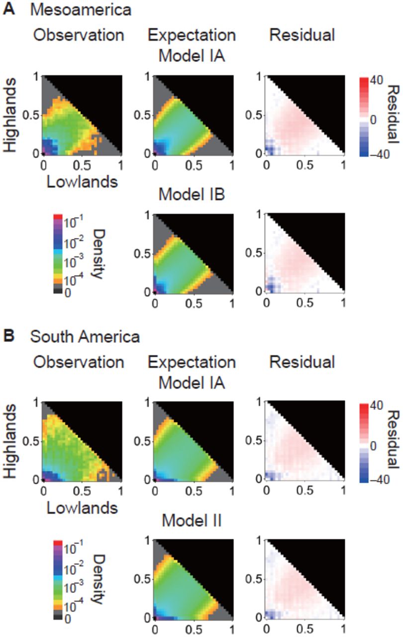
Estimated parameter values are listed in Figure 2 and Table 2; while the observed and expected JFDs were quite similar for both models, residuals indicated an excess of rare variants in the observed JFDs in all cases (Figure 3). Under both models IA and IB, we found expansion in the highland population in Mesoamerica to be unlikely, but a strong bottleneck followed by population expansion is supported in S. American highland maize in both models IA and II. The likelihood value of model IB was higher than the likelihood of model IA by 850 units of log-likelihood (Table 2), consistent with analyses suggesting that introgression from mexicana played a significant role during the spread of maize into the Mesoamerican highlands (Hufford et al. 2013).

Observed and expected joint distributions of minor allele frequencies in lowland and highland populations in (A) Mesoamerica and (B) S. America. Residuals are calculated as 
Estimated parameters of population size model
In addition to the parameters listed in Figure 2, we investigated the impact of varying the domestication bottleneck size (Nb). Surprisingly, Nb was estimated to be equal to NC, the population size at the end of the bottleneck, and the likelihood of Nb < Nc was much smaller than for alternative parameterizations (Table 2 and Table S2).
Comparisons of our empirical FST values to the null expectation simulated under our demographic models allowed us to identify significantly differentiated SNPs between lowland and highland populations. In all cases, observed FST values were quite similar to those generated under our null models (Figure S4), and model choice – including the parameterization of the domestication bottleneck – had little impact on the distribution of estimated P-values (Figure S5). We show resuits under Model IB for Mesoamerican populations and Model II for S. American populations. We chose P < 0.01 as an arbitrary cut-off for significant differentiation between lowland and highland populations, and identified 687 SNPs in Mesoamerica (687/76,989=0.89%) and 409 SNPs in S. America (409/63,160=0.65%) as significant outliers (Figure 4). Different cutoff values (0.05, 0.001) gave qualitatively identical results (data not shown). SNPs with significant FST P-values were enriched in intergenic regions rather than protein coding regions (60.0% vs. 47.9%, Fisher’s Exact Test P < 10−7 for Mesoamerica; 62.0% vs. 47.8%, FET P < 10−5 for S. America). Different cutoff values (0.05, 0.001) gave qualitatively identical results (data not shown).
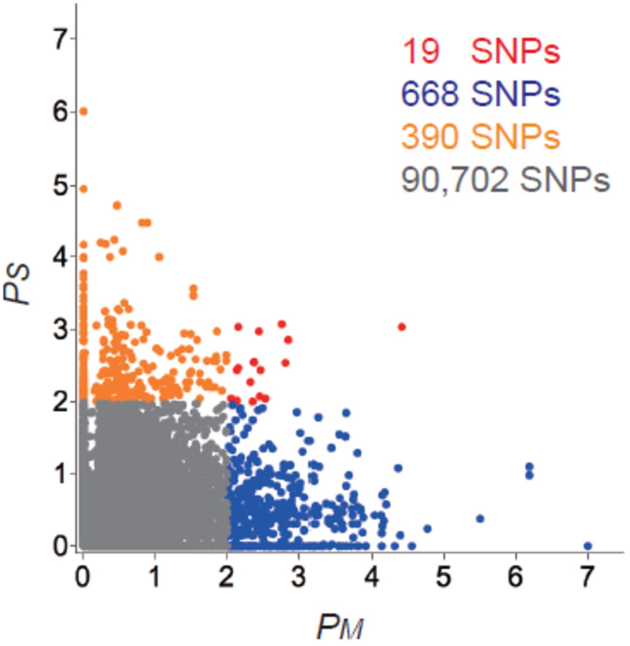
Scatter plot of – log10 P-values of observed FST values based on simulation from estimated demographic models. P-values are shown for each SNP in both Mesoamerica (Model IB; PM on x-axis) and S. America (Model II; PS on y-axis). Red, blue, orange and gray dots represents SNPs showing significance in both Mesoamerica and S. America, only in Mesoamerica, only in S. America, or in neither region, respectively (see text for details). The number of SNPs in each category is shown in the same color as the points.
Patterns of adaptation
Given the historical spread of maize from an origin in the lowlands, it is tempting to assume that the observation of significant population differentiation at a SNP should be primarily due to an increase in frequency of adaptive alleles in the highlands. To test this hypothesis, we sought to identify the adaptive allele at each locus using comparisons between Mesoamerica and S. America as well as to parviglumis. Alleles were called ancestral if they were at higher frequency in parviglumis, or uncalled in parviglumis but at higher frequency in all populations but one. SNPs were consistent with Mesoamerica-specific adaptation if one allele was at high frequency in one Mesoamerican population, low frequency in the other Mesoamerican population, and either: low frequency in parviglumis and at most intermediate frequency in S. American populations, or missing in parviglumis and at low frequency in S. American populations. On the other hand, SNPs were consistent with adaptation to highlands in both regions if they were at high frequency in both highland populations, and at low frequency in the lowland populations and parviglumis; and vice-versa for adaptation to lowlands in both regions. SNPs with an allele at high frequency in one highland and the alternate lowland population are suggestive of adaptation in both populations but on different haplotypes created by recombination.
Consistent with predictions, we infer that differentiation at 72.3% (264) and 76.7% (230) of SNPs in Mesoamerica and S. America is due to adaptation in the highlands after excluding SNPs with ambiguous patterns likely due to recombination. The majority of these SNPs show patterns of haplotype variation (by the PHS test) consistent with our inference of selection (Table S3 and Supporting Information, File S1).
Convergent evolution at the nucleotide level should be reflected in an excess of SNPs showing significant differentiation between lowland and highland populations in both Mesoamerica and S. America. Although the 19 SNPs showing FST P-values < 0.01 in both Mesoamerica (PM) and S. America (Ps) is statistically greater than the ≈ 5 expected (48,370 × 0.01 × 0.01 ≈ 4.8; χ2-test, P C 0.001), it nonetheless represents a small fraction (≈ 7 – 8%) of all SNPs showing evidence of selection. This paucity of shared selected SNPs does not appear to be due to our demographic model: a simple outlier approach based using the 1% highest FST values finds no shared adaptive SNPs between Mesoamerican and S. American highland populations. For 13 of 19 SNPs showing putative evidence of shared selection we could use data from parviglumis to infer whether these SNPs were likely selected in lowland or highland conditions (Supporting Information, File S1). Surprisingly, SNPs identified as shared adaptive variants more frequently showed segregation patterns consistent with lowland (10 SNPs) rather than highland adaptation (2 SNPs).
We also investigated how often different SNPs in the same gene may have been targeted by selection. To search for this pattern, we considered all SNPs within 10kb of a transcript as part of the same gene, though SNPs in an miRNA or second transcript within 10kb of the transcript of interest were excluded. We classified SNPs showing significant FST in Mesoamerica, S. America or in both regions into 778 genes. Of these, 485 and 277 genes showed Mesoamerica-specific and SA-specific significant SNPs, while 14 genes contained at least one SNP with a pattern of differentiation suggesting convergent evolution and 2 genes contained both Mesoamericaspecific and SA-specific significant SNPs. Overall, however, fewer genes showed evidence of convergent evolution than expected by chance (permutation test; P < 10−5). Despite similar phenotypes and environments, we thus see little evidence for convergent evolution at either the SNP or the gene level.
Comparison to theory
Given the limited empirical evidence for convergent evolution at the molecular level, we took advantage of recent theoretical efforts (Ralph and Coop 2014) to assess the degree of convergence expected under a spatially explicit population genetic model (see Materials and Methods). Our modeling estimates assume a maize population density ρ of the highlands to be around (0.5 ha field/person) × (0.5 people/km2) × (2 × 104 plants per ha field) = 5,000 plants per km2. The area of the Andean highlands currently under maize cultivation is estimated to be approximately A = 8400km2, giving a total maize population of Ap = 4.2 × 10⁷. Assuming an offspring variance of ξ2 = 30, we can then compute the waiting time Tmut = 1/λmut for a new beneficial mutation to appear and fix. We observe that even if there is relatively strong selection for an allele at high elevation (sb = 0.01), a single-base mutation with mutation rate μ = 10−8 would take an expected 3,571 generations to appear and fix. Our estimate of the maize population size uses the land area currently under cultivation and is likely an overestimate; Tmut scales linearly with the population size and lower estimates of A will thus increase Tmut proportionally. However, because Tmut also scales approximately linearly with both the selection coefficient and the mutation rate, strong selection and the existence of multiple equivalent mutable sites could reduce this time. For example, if any one of 10 sites within a gene could have equivalent strong selective benefit (sb = 0.1), Tmut would be reduced to 36 generations assuming constant A over time.
Gene flow between highland regions could also generate patterns of shared adaptive SNPs. From our demographic model we have estimated a mean dispersal distance of σ ≈ 1.8 kilometers per generation. With selection against the highland allele in low elevations 10−1 ≤ sm ≤ 10−4, the distance  over which the frequency of a highland-adaptive, lowland-deleterious allele decays into the lowlands is still short: between 7 and 250 kilometers. Since the Mesoamerican and Andean highlands are around 4,000 km apart, the time needed for a rare allele with weak selective cost sm = 10−4 in the lowlands to transit between the two highland regions is Tmig ≈ 8 × 10⁴ generations. While the exponential dependence on distance in equation (4) means that shorter distances could be transited more quickly, the waiting time Tmig is also strongly dependent on the magnitude of the deleterious selection coefficient: with sm = 10−4, Tmig ≈ 25 generations over a distance of 2,000 km, but increases to ≈ 108 generations with a still weak selective cost of sm = 10−3.
However, the rough calculations with coalescent theory above show that even neutral alleles are not expected to transit between the Mesoamerican and Andean highlands within 4,0 generations. This puts a lower bound on the time for deleterious alleles to transit as well, suggesting that we should not expect even weakly deleterious alleles (e.g. sm = 10−4) to have moved between highlands.
Taken together, these theoretical considerations suggest that any alleles beneficial in the highlands that are neutral or deleterious in the lowlands that are shared by both the Mesoamerican and S. American highlands would have been present as standing variation in both populations, rather than passed between them.
Alternative routes of adaptation
The lack of both empirical and theoretical support for convergent adaptation at SNPs or genes led us to investigate alternative patterns of adaptation.
We first sought to understand whether SNPs showing high differentiation between the lowlands and the highlands arose primarily via new mutations or were selected from standing genetic variation. We found that putatively adaptive variants identified in both Mesoamerica and S. America tended to segregate in the lowland population more often than other SNPs of similar mean allele frequency (85.3% vs. 74.8% in Mesoamerica (Fisher’s exact test P < 10−9 and 94.8% vs 87.4% in S. America, P < 10−4). We extended this analysis by retrieving SNP data from 14 parviglumis inbred lines included in the Hapmap v2 data set, using only SNPs with n > 10(Chia et al. 2012; Hufford et al. 2012b). Again we found that putatively adaptive variants were more likely to be polymorphic in parviglumis (78.3% vs. 72.2% in Mesoamerica (Fisher’s exact test P < G.Gl and 80.2% vs 72.8% in S. America, P < 0.01).
While maize in highland Mesoamerica grows in sympatry with the highland teosinte mexicana, maize in S. America is outside the range of wild Zea species, leading to a marked difference in the potential for adaptive introgression from wild relatives. Pyhäjärvi et al. (2013) recently investigated local adaptation in parviglumis and mexicana populations, characterizing differentiation between these subspecies using an outlier approach. Genome-wide, only a small proportion (2–7%) of our putatively adaptive SNPs were identified by Pyhäjärvi et al. (2013), though these numbers are still in excess of expectations (Fisher’s exact test P < 10−3 for S. America and P < 10−8 for Mesoamerica; Table S4). The proportion of putatively adaptive SNPs shared with teosinte was twice as high in Mesoamerica, however, leading us to evaluate the contribution of introgression from mexicana (Hufford et al. 2013) in patterning differences between S. American and Mesoamerican highlands.
The proportion of putatively adaptive SNPs in introgressed regions of the genome in highland maize in Mesoamerica was nearly four times higher than found in S. America (FET P < 11−11), while differences outside introgressed regions were much smaller (7.5% vs. 6.2%; Table S5). Furthermore, of the 77 regions identified as introgressed in Hufford et al. (2013), more than twice as many contain at least one FST outlier in Mesoamerica as in S. America (23 compared to 9, one-tailed Z-test P = 0.0027). Excluding putatively adaptive SNPs, mean FST between Mesoamerica and S. America is only slightly higher in introgressed regions (0.032) than across the rest of the genome (0.020), suggesting the enrichment of high FST SNPs seen in Mesoamerica is not simply due to neutral introgression of a divergent teosinte haplotype.
Discussion
Our analysis of diversity and population structure in maize landraces from Mesoamerica and S. America points to an independent origin of S. American highland maize, in line with earlier archaeological (Piperno 2006; Perry et al. 2006; Grobman et al. 2012) and genetic (van Heerwaarden et al. 2011) work. We use our genetic data to fit a model of historical population size change, and find no evidence of a bottleneck in Mesoamerica but a strong bottleneck followed by expansion in the highlands of S. America. Surprisingly, our models showed no support for a maize domestication bottleneck, apparently contradicting earlier work (Eyre-Walker et al. 1998; Tenaillon et al. 2004; Wright et al. 2005). One factor contributing to these differences is the set of loci sampled. Previous efforts focused on data exclusively from protein-coding regions, while our data set includes a large number of noncoding variants. Diversity differences between maize and teosinte are greatest in proteincoding regions (Hufford et al. 2012b), presumably due to the effects of background selection (Charlesworth et al. 1993), and demographic estimates using only protein-coding loci should thus overestimate the strength of a domestication bottleneck. While a more detailed comparison with data from teosinte will be required to validate these results, they nonetheless suggest the value of a reassessment of the combined impacts of demography and selection on genome-wide patterns of diversity during maize domestication.
We identified SNPs deviating from patterns of allele frequencies determined by our demographic model as loci putatively under selection for highland adaptation. These conclusions are supported by evidence of haplotype differentiation (Table S3) and the directionality of allele frequency change (Supporting Information, File S1). Consistent with results from both GWAS (Wallace et al. 2014) and local adaptation in teosinte (Pyhäjärvi et al. 2013), we find that putatively adaptive SNPs are enriched in intergenic regions of the genome, further suggesting an important role for regulatory variation in maize evolution.
Although our data identify hundreds of loci that may have been targeted by natural selection in Mesoamerica and S. America, fewer than 1.8% of SNPs and 2.1% of genes show evidence for convergent evolution between the two highland populations. This relative lack of convergent evolution is concordant with recently developed theory (Ralph and Coop 2014), which applied to this system suggests that convergent evolution involving identical nucleotide changes is quite unlikely to have occurred in the time since domestication through either recurrent mutation or migration across Central America via seed sharing. These results are generally robust to variation in most of the parameters, but are sensitive to gross misestimation of some of the parameters – for example if seed sharing was common over distances of hundreds of kilometers. The modeling highlights that our outlier approach may not detect traits undergoing convergent evolution if the genetic architecture of the trait is such that mutation at a large number of nucleotides would have equivalent effects on fitness (i.e. adaptive traits have a large mutational target). While QTL analysis suggests that some of the traits suggested to be adaptive in highland conditions may be determined by only a few loci (Lauter et al. 2004), others such as flowering time (Buckler et al. 2009) are likely to be the result of a large number of loci, each with small and perhaps similar effects on phenotype. Future quantitative genetic analysis of highland traits using genome-wide association methods may prove useful in searching for the signal of selection on such highly quantitative traits.
Our observation of little convergent evolution is also consistent with the possibility that much of the adaptation to highland environments made use of standing genetic variation in lowland populations. Indeed, we find that as much as 90% of the putatively adaptive variants in Mesoamerica and S. America are segregating in lowland populations, and the vast majority are also segregating in teosinte. Selection from standing variation should be common when the scaled mutation rate Θ (product of the effective population size, mutation rate and target size) is greater than 1, as long as the scaled selection coefficient Ns (product of the effective population size and selection coefficient) is reasonably large (Hermisson and Pennings 2005). Estimates of θ from synonymous nucleotide diversity in maize are around 0.014, (Tenaillon et al. 2004; Wright et al. 2005; Ross-Ibarra et al. 2009), suggesting that adaptation from standing genetic variation may be likely for target sizes larger than a few hundred nucleotides. In maize, such a scenario has been recently shown for the locus grassy tillers1 (Wills et al. 2013), at which adaptive variants in both an upstream control region and the 3’ UTR are segregating in teosinte but show evidence of recent selection in maize, presumably due to the effects of this locus on branching and ear number.
Finally, although we evaluated a genome-wide sample of more than 90,000 SNPs, this sampling is likely insufficient to capture all of the signals of selection across the genome. Linkage disequilibrium in maize decays rapidly (Chia et al. 2012), reaching a plateau in only a few hundred bp (Figure S6) and a much greater density of SNPs would be needed to effectively identify the majority of selective sweeps in the history of these populations (Tiffin and Ross-Ibarra 2014). SNP density alone does not explain the lack of convergent evolution seen at SNPs showing evidence of selection, however. Our genomic sampling may have thus identified only a subset of all loci targeted by natural selection, but there is no reason to believe that the percentage of selected loci showing convergent selection should change with higher genotyping density.
Acknowledgements
We appreciate the helpful comments of P. Morrell and members of the Ross-Ibarra lab and Coop lab. This project was supported by Agriculture and Food Research Initiative Competitive Grant 2009-01864 from the USDA National Institute of Food and Agriculture and funding from the National Science Foundation, grants IOS-1238014 (to JRI) and DBI-1262645 (to PLR).
Appendix
Demographic modeling
Throughout we use in many ways the branching process approximation – if an allele is locally rare, then for at least a few generations, the fates of each offspring are nearly independent. So, if the allele is locally deleterious, the total numbers of that allele behave as a subcritical branching process, destined for ultimate extinction. On the other hand, if the allele is advantageous, it will either die out or become locally common, with its fate determined in the first few generations. If the number of offspring of an individual with this allele is the random variable X with mean 𝔼[X] = 1 + s (selective advantage s > 0), variance Var [X] = ξ2, and ℙ {X = 0} > 0 (some chance of leaving no offspring), then the probability of local nonextinction p* is approximately p* ≈ 2s/ξ2 to a second order in s. The precise value can be found by defining the generating function Φ(u) = 𝔼[uX]; the probability of local nonextinction p* is the minimal solution to Φ(1 – u) = 1 – u. (This can be seen because: 1 – p* is the probability that an individual’s family dies out; this is equal to the probability that the families of all that individuals’ children die out; since each child’s family behaves independently, if the individual has x offspring, this is equal to (1 –p*)x; and Φ(1 – p*) = 𝔼[(1 – p*)X].)
If the selective advantage (s) depends on geographic location, a similar fact holds: index spatial location by i ϵ 1,&,n, and for u = (u1, u2,&, un) define the functions  where Xij is the (random) number of offspring that an individual at i produces at location j. Then p* = (p*1,…, p*n),the vector of probabilities that a new mutation at each location eventually fixes, is the minimal solution to Φ(1 – p*) = 1 – p*,i.e Φ1(1 – p*) = 1 – p*i.
Here we consider a linear habitat, so that the selection coefficient at location ℓi is si = min(sb, max(–sd, αℓi)). There does not seem to be a nice analytic expression for p* in this case, but since 1 – p* is a fixed point of Φ, the solution can be found by iteration: 1 – p* = limn→∞Φn(u) for an appropriate starting point u.
Maize model
The migration and reproduction dynamics we use are taken largely from van Heerwaarden et al. (2010). On a large scale, fields of N plants are replanted each year from Nf ears, either from completely new stock (with probability pe), from partially new stock (a proportion rm with probability pm), or entirely from the same field. Plants have an average of μE ears per plant, and ears have an average of N/Nf kernels; so a plant has on average μEN/Nf kernels, and a field has on average μEN ears and μEN2/Nf kernels. We suppose that a plant with the selected allele is pollen parent to (1 + s) μEN/Nf kernels, and also seed parent to (1 + s)μENN/Nf kernels, still in μE ears. The number of offspring a plant has depends on how many of its offspring kernels get replanted. Some proportion mg of the pollen-parent kernels are in other fields, and may be replanted; but with probability pe no other kernels (i.e. those in the same field) are replanted. Otherwise, with probability 1 – pm the farmer chooses Nf of the ears from this field to replant (or, (1 – rm)Nf/N) of them, with probability pm); this results in a mean number Nf/N(or, (1 – rm)Nf/N) of the plant’s ears of seed children being chosen, and a mean number 1 + s of the plant’s pollen children kernels being chosen. Furthermore, the field is used to completely (or partially) replant another’s field with chance pe/(1 – pe)(or pm); resulting in another Nf/N(or rmNf/N) ears and 1 + s(or rm(1 + s)) pollen children being replanted elsewhere. Here we have assumed that pollen is well-mixed within a field, and that the selected allele is locally rare. Finally, we must divide all these offspring numbers by 2, since we look at the offspring carrying a particular haplotype, not of the diploid plant’s genome.
The above gives mean values; to get a probability model we assume that every count is Poisson. In other words, we suppose that the number of pollen children is Poisson with random mean λP, and the number of seed children is a mixture of K independent Poissons with mean (1 + s)N/Nf each, where K is the random number of ears chosen to replant, which is itself Poisson with mean μK. By Poisson additivity, the numbers of local and migrant offspring are Poisson, with means λP = λPL + λPM and = μK = μKL + μKM respectively. With probability pe, λPM = mg(1 + s) and μK = λPL = 0. Otherwise, with probability (1 – pe)(1 – pm), μKL = Nf/N and λPL = (1 + s)(1 – mg); and with probability (1 – pe) = pm, = μKL (1 – rm)Nf/N and λPL = (1 – rm)(1 + s)(1 – mg). The migrant means are, with probability (1 – pe)pe/(1 – pe) = pe, μKM = Nf/N and λPM = 1 + s; while with probability (1 – pe)pm, μKM = rmNf/N and λPM = (1 + s)(rm(1 – mg) + mg), and otherwise μKM = 0 and λPM = mg(1 + s).
Parameter estimates used in calculations, and other notation.
Math
The generating function of a Poisson with mean λ is ϕ(u; λ) = exp(λ(u – 1)), and the generating function of a Poisson(μ) sum of Poisson(λ) values is ϕ((ϕ; u λ);μ). Therefore, the generating function for the diploid process, ignoring spatial structure, is


To get the generating function for a haploid, replace every instance of 1 + s by (1 + s)/2. As a quick check, the mean total number of offspring of a diploid is


We show numerically later that the probability of establishment is very close to 2s over the variance in reproductive number (as expected). It is possible to write down an expression for the variance, but the exact expression does not aid the intuition.
Migration and spatial structure
To incorporate spatial structure, suppose that the locations ℓk are arranged in a regular grid, so that ℓk = ak. Recall that sk is the selection coefficient at location k. If the total number of offspring produced by an individual at li is Poisson(λi), with each offspring independently migrating to location j with probability mij, then the number of offspring at j is Poisson(mijλi), and so the generating function is


We can then substitute this expression into equation (A1), with appropriate migration kernels for pollen and seed dispersal.For migration, we need migration rates and migration distances for both wind-blown pollen and for farmer seed exchange. The rates are parameterized as above; we need the typical dispersal distances, however. One option is to say that the typical distance between villages is dv, and that villages are discrete demes, so that pollen stays within the deme (pollen migration distance 0) and seed is exchanged with others from nearby villages; on average σs distance away in a random direction. The number of villages away the seed comes from could be geometric (including the possibility of coming from the same village).
0.1 Dispersal distance
The dispersal distance – the mean distance between parent and offspring – is equal to the chance of inter-village movement multiplied by the mean distance moved. This is
 at the parameter values above.
Iterating the generating function above finds the probability of establishment as a function of distance along the cline. This is shown in figure A1. Note that the approximation 2s divided by the variance in offspring number is quite close.

Probability of establishment, as a function of distance along and around an altitudinal cline, whose boundaries are marked by the green lines. (A) The parameters above; with cline width 62km; (B) the same, except with cline width 500km.
In the main text, we used a rough upper bound on the rate of migration that ignored correlations in migrants. As we show in Ralph and Coop (2014), the rate of adaptation by diffusive migration is more precisely

First note that for 10−1 ≤ sm ≤ 10−4, the value  is between 2 and 70 – so the exponential decay of the chance of migration falls off on a scale of between 2 and 70 times the dispersal distance. Above we have estimated the dispersal distance to be σ ≈ 3.5 km, and far below the mean distance σs to the field that a farmer replants seed from, when this happens, which we have as σs = 50 km. Taking σ = 3.5 km, we have that
  . A very conservative upper bound might be σ ≤ σs/10 (if farmers replaced 10% of their seed with long-distance seed every year). At this upper bound, we would have
  , which is not very different. This makes the exponential term small since R is on the order of thousands of kilometers.
Taking σ = 3.5 km, we then compute that if sm = 10−4 (very weak selection in the lowlands), then for R = 1,000 km, the migration rate is λmig ≤ 10−5, i.e. it would take on the order of 100,000 generations (years) to get a successful migrant only 1,000 km away, under this model of undirected, diffusive dispersal. For larger sm, the migration rate is much smaller.


